

概述
这一章的核心是:
SQL 查询不会直接在磁盘文件上执行。数据库系统会先把查询翻译成关系代数表达式,再经过优化器选择具体执行计划,最后由执行引擎按计划访问数据并返回结果。
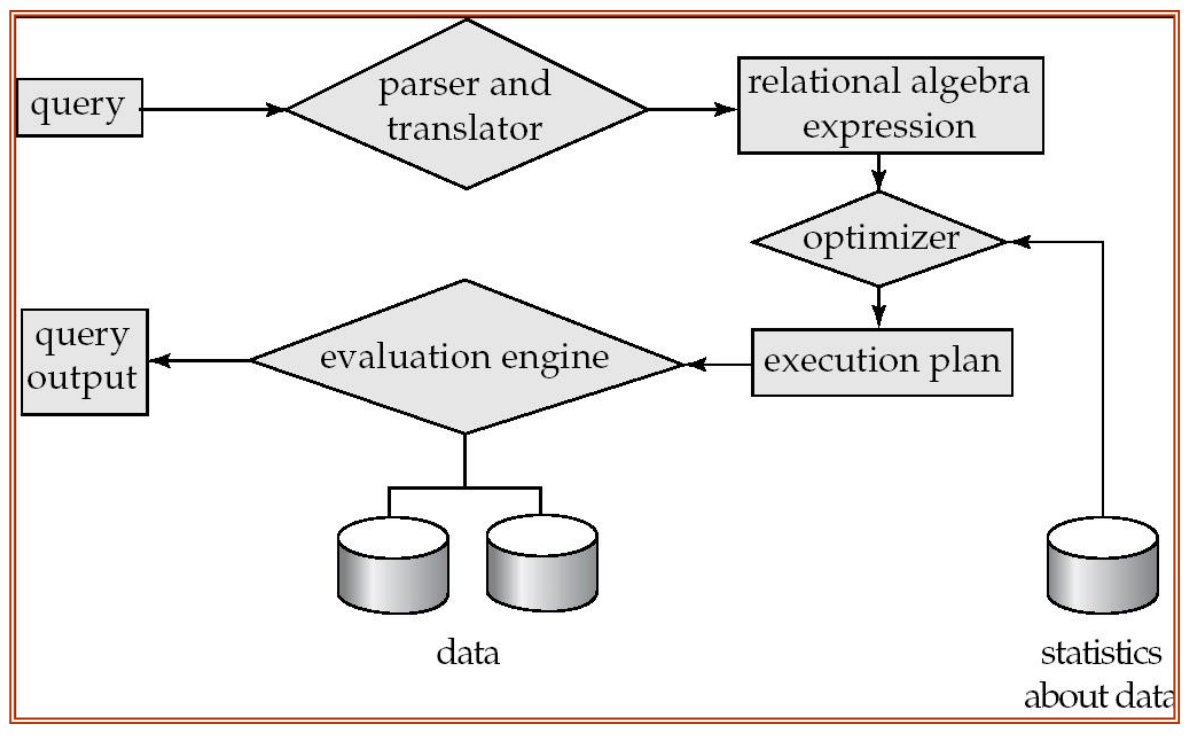
查询处理的基本链条是:
SQL query -> parser and translator -> relational algebra expression -> optimizer -> execution plan -> evaluation engine -> query output这一章主要解决两个问题:
- 一个关系代数操作怎么执行,例如 selection、sort、join、aggregation;
- 一棵表达式树怎么整体执行,例如 materialization 和 pipelining。
本章重点是各种算法的 I/O cost。
为了简化分析,通常只统计:
- block transfer 数量
- seek 数量
然后用下面公式估算代价:
其中:
- :block transfers 数量
- :seeks 数量
- :传输一个 block 的时间
- :一次 seek 的时间
目录
- 概述
- 目录
- Basic Steps in Query Processing
- Measures of Query Cost
- Selection Operation
- Sorting
- Join Operation
- Other Operations
- Evaluation of Expressions
- Query Processing in Memory
Basic Steps in Query Processing
Parsing and Translation
第一步是把用户写的 SQL 查询翻译成数据库内部表示。
具体做两件事:
- parse:检查 SQL 语法是否正确;
- verify:检查查询中引用的 relation、attribute 是否存在。
之后,系统会把查询翻译成关系代数表达式。
SQL 查询:
select name, titlefrom instructor natural join (teaches natural join course)where dept_name = 'Music' and year = 2009;可以翻译成关系代数表达式:
这个表达式只是逻辑层面的表示,还没有决定具体怎么扫表、用哪个索引、采用哪种 join 算法。
Optimization
同一个 SQL 查询可以对应多个等价的关系代数表达式,也可以对应多个不同的物理执行计划。
优化器的任务是:
在所有等价的 evaluation plans 中,选择估计代价最低的计划。
优化包括两层:
- 逻辑优化:改变关系代数表达式结构,例如 selection pushdown。
- 物理优化:为每个操作选择具体算法,例如 index scan、hash join、merge join。
上面的查询可以从初始表达式树变成更好的表达式树:
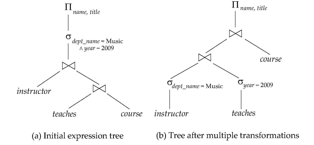 核心思想是:
越早过滤,后续 join 的输入越小。
Evaluation
最后一步是执行。
查询执行引擎接收 optimizer 产生的 query-evaluation plan,按计划运行各个操作,访问存储系统并返回结果。
Evaluation Plan
evaluation plan 指明了:
- 每个关系代数操作采用什么算法;
- 操作之间如何协调;
- 中间结果是物化到磁盘,还是通过 pipeline 直接传给父操作;
- 是否使用索引、排序、hash table 等物理结构。
同一个逻辑表达式可以有不同的物理计划:
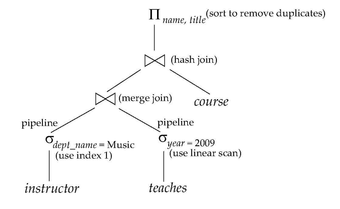
这里不仅说明了有 selection / join / projection,还说明了:
instructor上的 selection 使用 index;teaches上的 selection 使用 linear scan;- 下层 join 使用 merge join;
- 上层 join 使用 hash join;
- projection 后还需要 sort 去重。
EXPLAIN
大多数数据库支持查看优化器选出的执行计划。
常见命令:
EXPLAIN <query>;它通常显示:
- optimizer 选择的 plan;
- 每个操作的 cost estimate;
- 使用的 index / scan / join algorithm。
不同数据库语法略有不同:
- Oracle:
explain plan for <query>,再查询dbms_xplan.display; - SQL Server:
set showplan_text on; - PostgreSQL:
EXPLAIN <query>和EXPLAIN ANALYZE <query>。
EXPLAIN ANALYZE 会真正执行查询,并显示实际运行统计信息。
PostgreSQL 中的 cost 常写成:
startup_cost..total_cost含义是:
startup_cost:产生第一条 tuple 前的代价;total_cost:产生全部结果的总代价。
Measures of Query Cost
代价模型
查询总代价通常可以从多个角度衡量:
- disk accesses
- CPU time
- network communication
- memory usage
但在传统数据库代价模型中,磁盘 I/O 通常是主导因素,也比较容易估计。
所以本章简化为:
Cost = block transfer cost + seek cost即:
这里:
- :传输一个 block 的时间;
- :一次 seek 的时间。
典型值:
| 存储介质 | 直观理解 | ||
|---|---|---|---|
| 高端磁盘 | 约 4 ms | 约 0.1 ms | seek 远比顺序传输贵 |
| SSD | 约 20-90 μs | 约 2-10 μs | random access 仍贵,但差距变小 |
NOTE本章公式通常忽略 CPU cost 和最终输出写盘 cost。
真实数据库系统会把 CPU、内存、并发、网络等因素也纳入优化器代价模型。这里只是为了推导算法代价,先抓最主要的 I/O 因素。
buffer 对代价估计的影响
很多算法都能利用额外 buffer 降低 I/O。
但可用内存大小受下面因素影响:
- 系统总内存;
- buffer pool 当前状态;
- 其他并发查询;
- 操作系统进程;
- 数据是否已经在 buffer 中。
因此,代价估计常常使用保守假设:
只假设操作拥有它执行所需的最小 buffer。
如果实际运行时数据已经在 buffer 中,真实代价可能显著低于估计代价。
Selection Operation
selection 的目标是从 relation 中找出满足条件的 tuple。
例如:
select *from instructorwhere dept_name = 'Music';对应关系代数:
selection 的核心问题是:
怎样少读磁盘块,就找到满足条件的 tuple?
记号:
- :关系;
- :关系 占用的 block 数;
- :关系 中 tuple 数;
- :B+-tree index 从 root 到 leaf 需要访问的 index block 数;
- :满足条件的记录所在 data block 数;
- :存放 matching pointers 的 index block 数;
- :matching records 数。
TIP理解 selection 算法时,先区分三件事:
- 能不能用 index:条件是否作用在 index search key 上;
- 结果有几条:条件属性是不是 key;
- 结果在磁盘上是否连续:index 是 clustering 还是 secondary。
很多代价公式的差别,都来自这三点。
File Scan
A1 Linear Search
最直接的方法是线性扫描整个文件。
算法:
scan every block of relation r test every tuple output tuple if it satisfies the selection condition最坏代价:
原因是:
- 先 seek 到 relation 的第一个 block;
- 然后顺序读完整个 relation,共读 个 blocks。
如果 selection 条件是 key equality,找到记录后可以停止。
平均代价:
因为如果目标记录均匀分布,平均扫半张表就能找到。
假设 student 有 100 个 blocks,查询:
select *from studentwhere ID = '12345';如果没有 ID 上的索引,只能从第一个 block 开始扫描。
- 最坏情况:目标记录在最后一个 block,读 100 个 blocks;
- 平均情况:目标记录大约在中间,读 50 个 blocks。
所以 key equality 虽然只返回一条 tuple,但没有 index 时仍可能很慢。
linear search 的优点是适用性最强:
- 不要求文件有序;
- 不要求有 index;
- 可以处理任意 selection condition。
WARNING普通文件上的 binary search 通常不划算。
二分查找要求能快速跳到中间位置,但磁盘上的数据块未必连续,每次跳转可能都是一次 seek。对于磁盘来说,多次随机 seek 往往比一次顺序扫描更贵。
所以除非有索引,否则直接对数据文件做 binary search 通常不是好方案。
Index Scan
index scan 使用索引来定位 tuple。
前提是:
selection condition 必须作用在 index 的 search key 上。
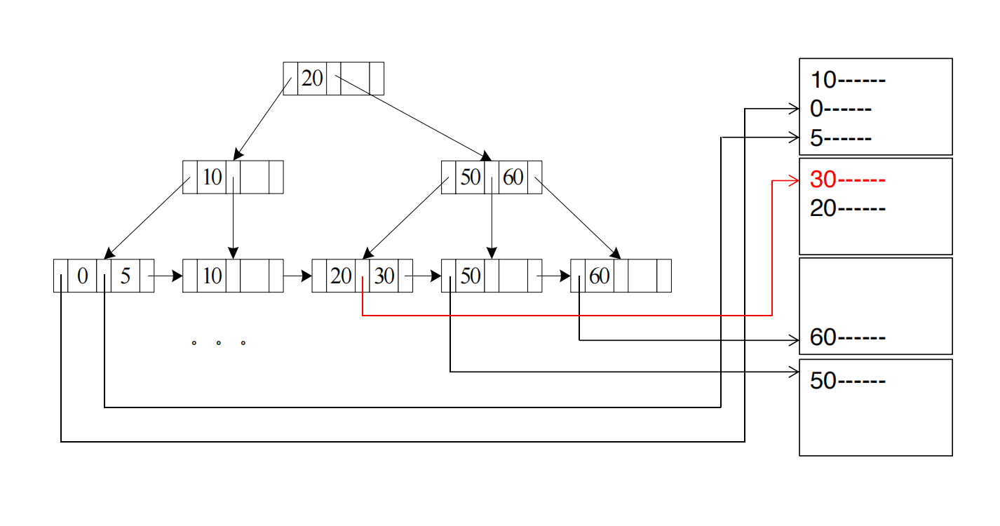
clustering index:
- clustering index:数据文件本身按 index search key 的顺序存放,或者至少相近值尽量放在一起;
- secondary index:index leaf 按 search key 排序,但数据文件本身不按这个 search key 排序。
假设 index 建在属性 A 上。
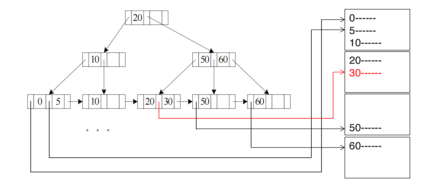
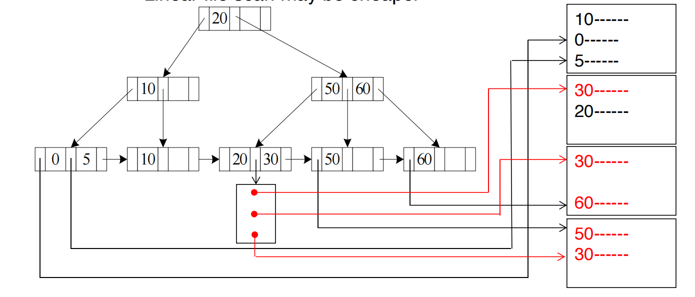
clustering index 的数据文件可能是:
A: 0, 5, 10, 20, 30, 30, 30, 50, 60secondary index 的数据文件可能是:
A: 10, 30, 5, 60, 30, 0, 50, 30两者都能通过 B+ 树找到记录。区别在于:
- clustering index 中,相同或相近的
A值通常连续; - secondary index 中,满足条件的记录可能散落在很多 data blocks 中。
A2 Clustering B+-tree Index, Equality on Key
条件形式:
其中 是 key,并且有 primary / clustering B+-tree index。
由于 key 唯一,只会返回一条记录。
代价:
含义:
- 访问 B+ 树从 root 到 leaf,共 个 index blocks;
- leaf entry 中有指向真实记录的 pointer;
- 再访问 1 个 data block。
假设要查:
select *from rwhere A = 30;B+ 树查找过程可以理解成:
root block -> internal block -> leaf block containing 30 -> data block containing the actual tuple如果 ,则大约访问:
3 个 index blocks + 1 个 data block = 4 个 blocks因为这些 block 在磁盘上不保证连续,所以按每个 block 一次随机 I/O 估计:
真实系统中 root 和上层 internal nodes 往往在 buffer 中,所以实际代价可能更小。
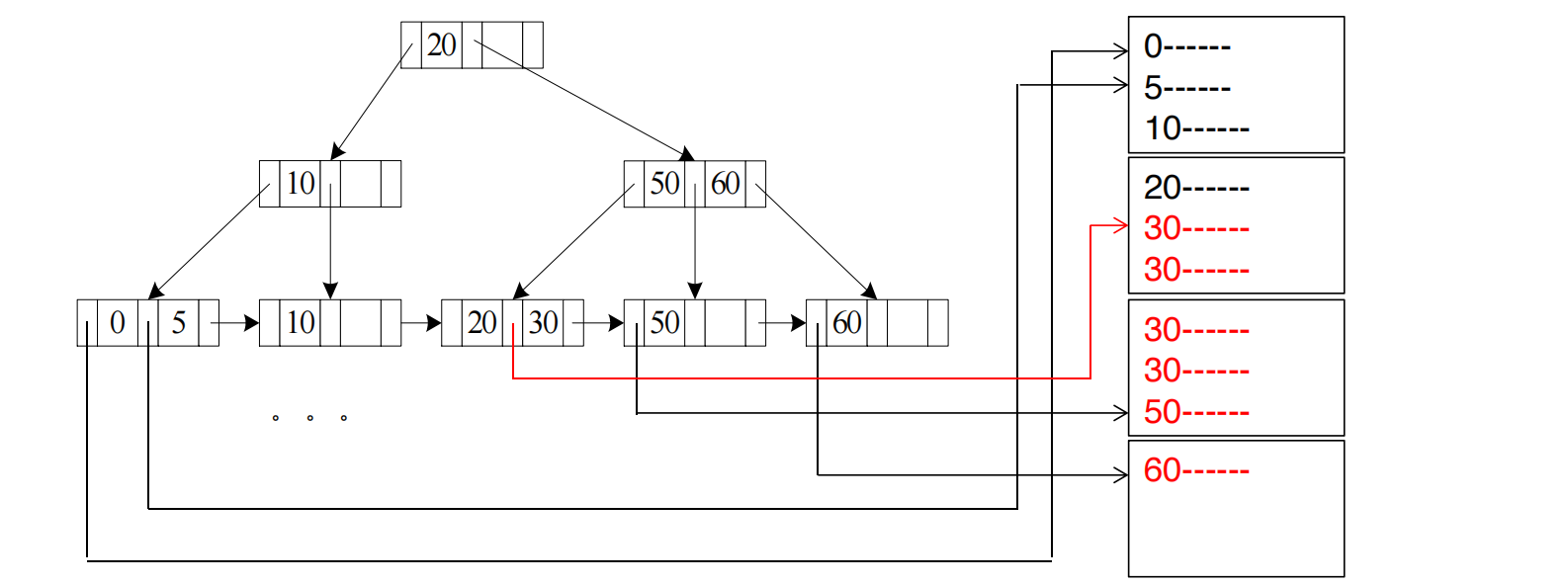
A3 Clustering B+-tree Index, Equality on Nonkey
条件仍然是 equality,但属性不是 key。
这时 可能返回多条记录。
因为是 clustering index,满足条件的记录在数据文件中通常连续存放。
设匹配记录占 个连续 data blocks,代价为:
公式分解:
h_i(t_T+t_S) : 走 B+ 树,从 root 到 leaf,找到第一个 v+t_S : seek 到第一个匹配 data block+b*t_T : 顺序读 b 个连续 data blocks假设 dept_name 不是 key,很多教师都属于 Music 系。
select *from instructorwhere dept_name = 'Music';如果 instructor 文件按 dept_name 聚集存放,那么数据可能是:
Biology ...Comp. Sci. ...Music, Music, Music, Music ...Physics ...B+ 树只负责帮你找到第一条 Music。
找到之后,不需要每条记录都随机跳一次。因为所有 Music 记录基本连续,直接顺序读这一段即可。
这就是为什么后半部分是:
不是:
A4 Secondary B+-tree Index, Equality on Key
如果是 secondary B+-tree index,但 equality 条件作用在 key 上,则也只返回一条记录。
代价与 A2 相同:
区别在于:
- secondary index 的顺序和数据文件物理顺序不同;
- 但 key equality 只取一条记录,所以只会根据 pointer 跳到一个 data block。
假设数据文件按 ID 排序,但我们在 email 上建了 secondary index。
select *from studentwhere email = 'a@zju.edu.cn';如果 email 是 key,那么只匹配一个学生。
虽然数据文件不是按 email 排的,但 index leaf 中的 pointer 会直接指向那条 student record。
所以流程仍是:
查 B+ 树 email index -> 找到 pointer -> 读 1 个 data block不会因为是 secondary index 就找不到。
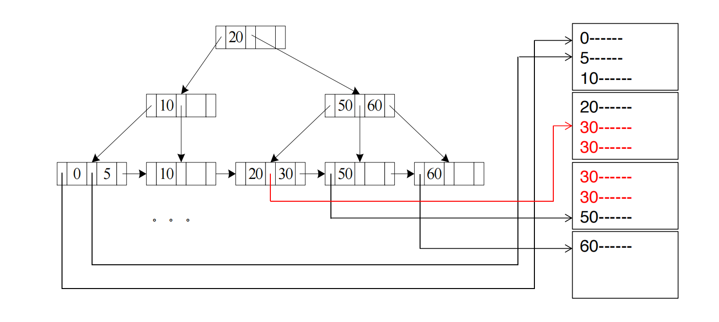
A4’ Secondary B+-tree Index, Equality on Nonkey
这是很容易变贵的一种情况。
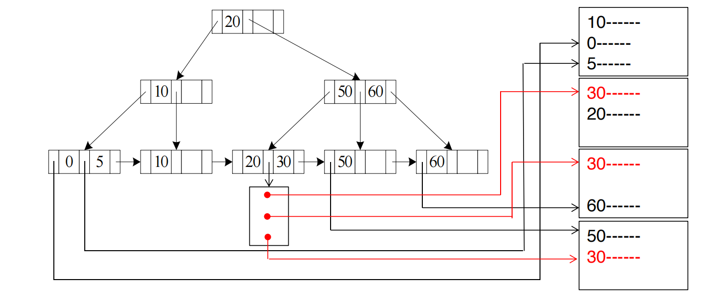
条件作用在 nonkey 上,可能返回 条记录;这些记录在数据文件中未必连续。
设:
- :matching pointers 存放在 个 index blocks 中;
- :matching records 数量。
代价估计:
公式分解:
h_i : 走 B+ 树到 leafm : 读取存放 matching pointers 的 index blocksn : 根据 n 个 pointers 取 n 条真实记录最贵的是最后的 。
因为 secondary index 不决定数据文件的物理顺序,所以这 条真实记录可能分散在 个不同 data blocks 中。
假设数据文件按 ID 排序,但有一个 secondary index 建在 dept_name 上。
select *from instructorwhere dept_name = 'Music';索引中 Music 的 pointer 可能是:
Music -> ptr(record 18), ptr(record 203), ptr(record 967), ptr(record 1802)这些真实记录在数据文件中可能分布在完全不同的位置:
block 2, block 40, block 190, block 350于是每取一条记录都可能要随机 I/O。
这就是 secondary index on nonkey 可能很差的原因。
WARNINGsecondary index on nonkey 在匹配结果很多时可能非常差。
如果匹配了表中 30% 的记录,使用 secondary index 可能产生大量随机 I/O。此时一次 linear file scan 反而可能更便宜。
Selections Involving Comparisons
比较条件包括:
范围查询的核心问题是:
满足条件的记录能不能连续读?
A5 Clustering B+-tree Index, Comparison
如果 relation 按 排序,并且有 clustering index:
- 对于 :用 index 找到第一条 的 tuple,然后顺序扫描后面的记录;
- 对于 :从 relation 开头开始顺序扫描,直到第一条 的 tuple。
对于 ,代价与 A3 类似:
这里 是满足范围条件的记录所在 block 数。
假设文件按 A 排序:
0, 5, 10, 20, 30, 30, 30, 50, 60查询:
where A >= 30流程是:
1. 用 B+ 树找到第一个 A >= 30 的位置2. 跳到这个 data block3. 从 30 开始顺序读到文件末尾如果满足条件的记录在 4 个连续 blocks 中,那么读数据部分是:
因为定位一次后可以连续读。
NOTE为什么 常常不使用 index?
如果文件本身已经按 排序,查询:
满足条件的记录在文件开头:
直接从文件开头顺序扫到第一个大于 30 的记录即可。
使用 index 只能帮你找到边界,但仍然要读前面那一大段,反而多了索引访问成本。
A6 Secondary B+-tree Index, Comparison
如果使用 secondary index 处理范围查询:
- 对于 :找到第一条 index entry,再顺序扫描 leaf entries;
- 对于 :从 index leaf 开始扫到第一条 ;
- 对每个 pointer 再去数据文件中取实际记录。
问题是:
index leaf 中的 entries 是连续的,但它们指向的数据记录不一定连续。
假设 secondary index 上满足 A >= 30 的 entries 连续:
30 -> ptr(block 20)31 -> ptr(block 2)32 -> ptr(block 88)33 -> ptr(block 7)扫描 index leaf 很顺序,但取真实 records 时要跳到很多不同 data blocks。
所以如果范围很大,A6 可能比 linear scan 更差。
Implementation of Complex Selections
复杂 selection 条件通常由 conjunction、disjunction、negation 构成。
A7 Conjunctive Selection Using One Index
条件形式:
做法:
- 从多个简单条件中选择一个最适合使用 index 的 ;
- 用 A1-A6 中代价最低的算法取出候选 tuple;
- 在内存中测试剩余条件。
核心思想:
先用最有选择性的条件缩小候选集。
查询:
select *from instructorwhere dept_name = 'Music' and salary > 90000;假设只有 dept_name 上有 index。
做法是:
1. 用 dept_name index 找出 Music 系教师2. 把这些 tuple 读入内存3. 在内存中继续检查 salary > 90000如果 Music 系只有 20 人,而全校有 2000 名教师,这个 index 就很有用。
如果 Music 系有 1000 人,而 salary > 90000 只有 10 人,但 salary 没有 index,系统仍只能先用 dept_name index 再过滤。
A8 Conjunctive Selection Using Composite Index
如果存在 composite index,例如:
(dept_name, salary)那么查询:
where dept_name = 'Finance' and salary = 80000可以直接用复合索引定位同时满足两个条件的记录。
单属性索引方案:
dept_name index -> 找到所有 Finance 教师salary index -> 找到所有工资 80000 的教师然后取交集复合索引方案:
(dept_name, salary) index -> 直接找 ('Finance', 80000)复合索引通常更直接,候选集更小。
WARNING复合索引有顺序。
索引
(dept_name, salary)对下面查询很有效:但对下面查询未必高效:
原因是 B+ 树按 lexicographic order 排序。一旦第一个属性是范围条件,第二个属性通常难以继续精确定位。
A9 Conjunctive Selection by Intersection of Identifiers
如果每个条件都有相应索引,并且索引返回 record pointer 或 record id:
- 对每个条件分别用索引得到 pointer 集合;
- 对这些集合取交集;
- 再根据交集中的 pointer 访问数据记录;
- 没有索引的条件在内存中检查。
适合情况:
- 多个条件都有索引;
- 单个条件选择性一般,但交集很小。
查询:
where dept_name = 'Finance' and salary = 80000假设只有两个单属性索引。
dept_name='Finance' -> {r1, r3, r8, r20}salary=80000 -> {r2, r3, r20, r50}intersection -> {r3, r20}最后只需要访问 r3 和 r20 对应的数据记录。
A10 Disjunctive Selection by Union of Identifiers
条件形式:
只有当所有条件都有可用索引时,才适合用 union of identifiers。
做法:
- 对每个条件分别用索引得到 pointer 集合;
- 对这些集合取并集;
- 根据 pointer 取记录。
查询:
where dept_name = 'Music' or salary > 100000如果两个条件都有索引:
dept_name='Music' -> {r1, r7, r9}salary>100000 -> {r2, r7, r20}union -> {r1, r2, r7, r9, r20}注意 r7 只输出一次。
如果有任一条件没有可用索引,通常退化成 linear scan。
原因是:
A or B只要 B 没有索引,就无法只靠索引找全所有满足 B 的 tuple,最终仍要扫表。
Negation
条件形式:
通常用 linear scan。
查询:
where dept_name <> 'Music'即使 dept_name 上有 index,也通常不适合用 index。
原因是满足 dept_name <> 'Music' 的记录可能占绝大多数。用 index 会得到大量 pointers,然后随机访问大量 data blocks,不如直接顺序扫描全表。
如果满足 的记录极少,且 上有可用索引,也可以考虑利用索引间接处理。但一般情况下,否定条件对索引不友好。
Bitmap Index Scan
PostgreSQL 的 bitmap index scan 用来弥合两种极端:
- secondary index scan:匹配少时很好,匹配多时可能大量随机 I/O;
- linear file scan:匹配多时稳定,匹配少时浪费。
基本思想:
先用 index 找到满足条件的 record ids,再用 bitmap 汇总这些 records 所在的 data pages,最后按 page 读取数据。
bitmap 的粒度是 page / block:
1 bit per page步骤:
- 用 index scan 找到满足条件的 record ids;
- 根据 record id 找到其所在 page,并把 bitmap 中对应 bit 置为 1;
- 再扫描或访问 relation,只读取 bit 为 1 的 pages。
假设 relation 有 8 个 pages:
page: 0 1 2 3 4 5 6 7bitmap: 0 1 0 1 0 0 1 0表示只需要读取 page 1、page 3、page 6。
如果 index 返回很多 records,但它们集中在少数 pages 上,bitmap scan 可以避免对同一个 page 重复随机访问。
性能特点:
- 如果只有少量 bit 为 1,表现接近 index scan;
- 如果大多数 bit 为 1,表现接近 linear scan;
- 一般不会比两种极端方案差很多。
TIP这里的 bitmap index scan 和 Chapter 14 中的 bitmap index 不完全一样。
- bitmap index 是一种索引结构;
- bitmap index scan 是 PostgreSQL 的一种执行策略,用 bitmap 收集将要访问的 data pages。
Sorting
排序在数据库系统中很重要,原因有两个:
- SQL 查询可能要求排序输出,例如
ORDER BY; - 很多操作依赖排序,例如 duplicate elimination、merge join、aggregation。
如果 relation 能放进内存,可以使用 quicksort 等内存排序算法。
如果 relation 放不进内存,则需要 external sorting。
直接通过 index 读出有序数据也可行,但如果 index 是 secondary index,可能导致每条 tuple 一次随机 I/O,代价很高。
假设数据文件没有按 salary 排序,但有一个 secondary index on salary。
执行:
select *from instructororder by salary;可以沿着 salary index 的 leaf nodes 读出有序 pointer。
但每个 pointer 指向的数据记录可能在不同 data block 中。于是为了输出完整 tuple,可能每条 tuple 都触发一次随机 I/O。
所以“有索引能得到顺序”不等于“一定便宜”。
External Sort-Merge
外部排序最常用的是 external sort-merge。
设:
- :可用内存页数;
- :relation 的 block 数。
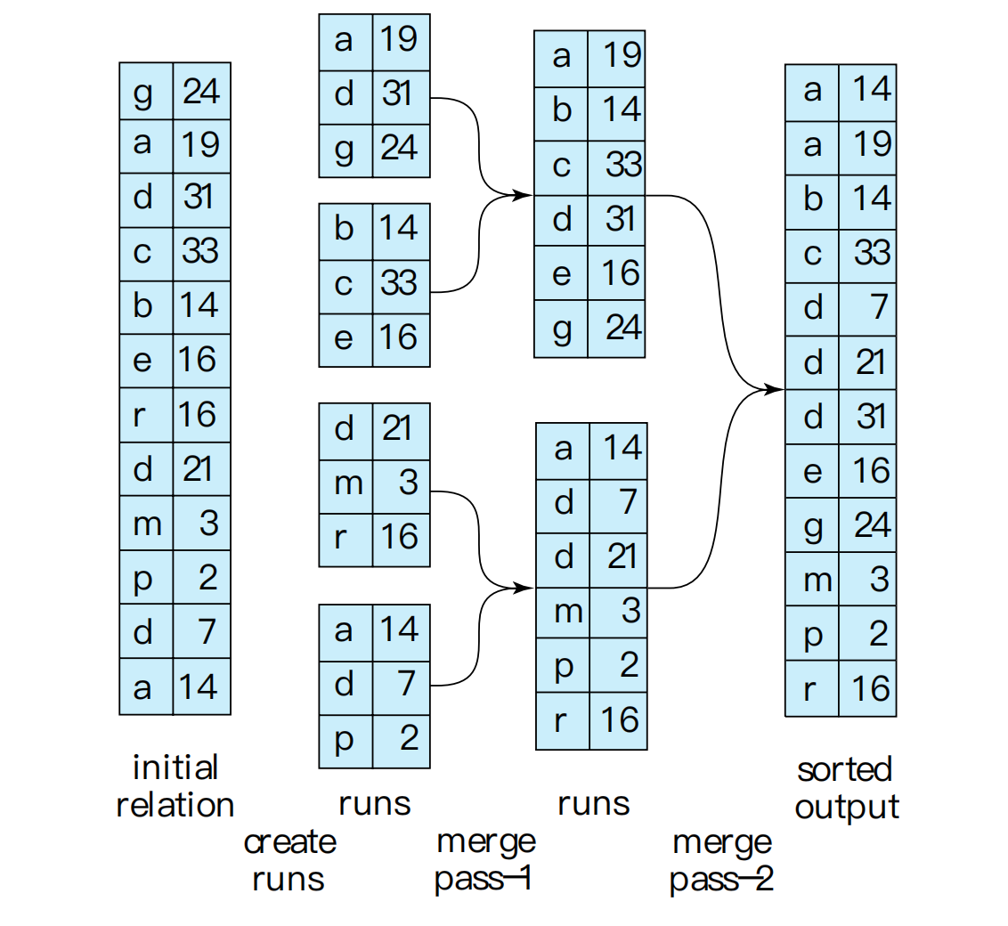
算法分两阶段:
Phase 1: create sorted runsPhase 2: merge runs直观理解:
内存一次只能装一小段,就先把每一小段内部排好序;然后像归并排序一样,把很多有序小段合成一个全局有序文件。
Create Sorted Runs
先创建初始有序归并段。
i = 0repeat until end of relation: read M blocks into memory sort these blocks in memory write sorted data to run R_i i = i + 1总 run 数为:
每个 run 内部有序。
假设:
b_r = 1000 blocksM = 100 pages一次能读 100 个 blocks 到内存排序。
所以初始 run 数:
得到:
R0: 第 1-100 blocks 排好序R1: 第 101-200 blocks 排好序...R9: 第 901-1000 blocks 排好序注意:每个 run 内部有序,但不同 runs 之间还没有整体有序。
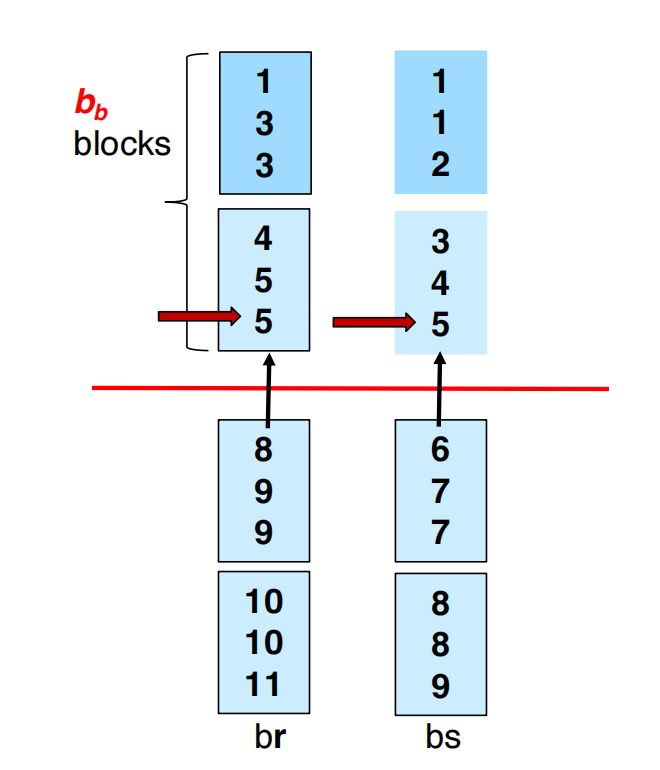
Merge Runs
如果:
则一次 merge pass 就够。
内存分配:
- 个 buffer pages 分别给 个 input runs;
- 1 个 output buffer page。
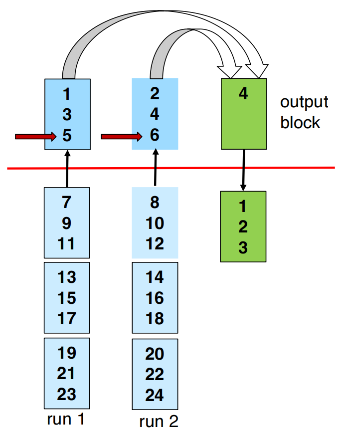
merge 过程:
read first block of each run into memoryrepeat: choose smallest tuple among input buffer pages write it to output buffer delete it from its input buffer if an input buffer becomes empty: read next block of that rununtil all input buffers are empty假设有两个有序 runs:
run 1: 1, 4, 9, 13run 2: 2, 3, 10, 11merge 时维护两个指针:
run1 指向 1run2 指向 2比较指针所指元素:
1 < 2,输出 1,run1 指针后移到 42 < 4,输出 2,run2 指针后移到 33 < 4,输出 3,run2 指针后移到 104 < 10,输出 4,run1 指针后移到 9...最后得到:
1, 2, 3, 4, 9, 10, 11, 13多路 merge 和这个逻辑一样,只是从多个 input buffers 的当前最小 tuple 中选最小者。
如果:
则需要多轮 merge。
每一轮最多合并:
个 runs,因为还要保留 1 个 output buffer。
每一轮会让 run 数大约缩小 倍,直到只剩一个最终有序 run。
如果 ,初始有 90 个 runs。
每一轮最多合并 10 个 runs,所以一轮后 run 数变成:
这时 9 个 runs 小于 11 个 buffer pages,下一轮就能合并成最终结果。
过程是:
90 runs --pass 1--> 9 larger runs --pass 2--> 1 final sorted runCost of External Sort-Merge
设 merge pass 数为:
更精确地说,括号内可写成初始 run 数 。
block transfer cost
创建初始 runs:
- 读 relation:;
- 写初始 runs:。
代价:
每个 merge pass 也要读写所有数据。
但最终输出写盘通常不计入操作代价,因为结果可能直接传给父操作。
所以总 block transfers:
即:
假设:
b_r = 1000M = 100初始 runs:
如果 ,一次 merge 能合并 99 个 runs,因此:
总 block transfers:
对应过程:
读原 relation 1000写初始 runs 1000merge 时读初始 runs 1000最终输出写盘不计seek cost
simple version 中,每次只按一个 block 读写。
创建初始 runs 的 seeks:
原因是每个初始 run:
读一段连续 blocks:1 次 seek写一个 sorted run:1 次 seek初始 run 数是 ,所以乘 2。
merge 阶段的 seeks:
理由:
- 每个普通 merge pass 读 blocks、写 blocks,simple version 近似为 次 seeks;
- 最后一轮最终输出不计写盘,所以少算一次写 的 seeks。
因此总 seeks:
继续设:
b_r = 1000M = 100P = 1创建初始 runs 的 seeks:
merge 阶段:
总 seeks:
这个数字看起来大,是因为 simple version 假设 merge 时每次只读写 1 个 block,导致频繁 seek。
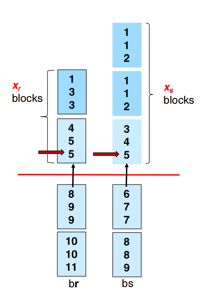
advanced version
simple version 的问题是:
merge 时每个 run 只分配 1 个 buffer block,会导致 seeks 过多。
改进做法:给每个 run 分配 个 buffer blocks。
这样每次可以连续读写 个 blocks。
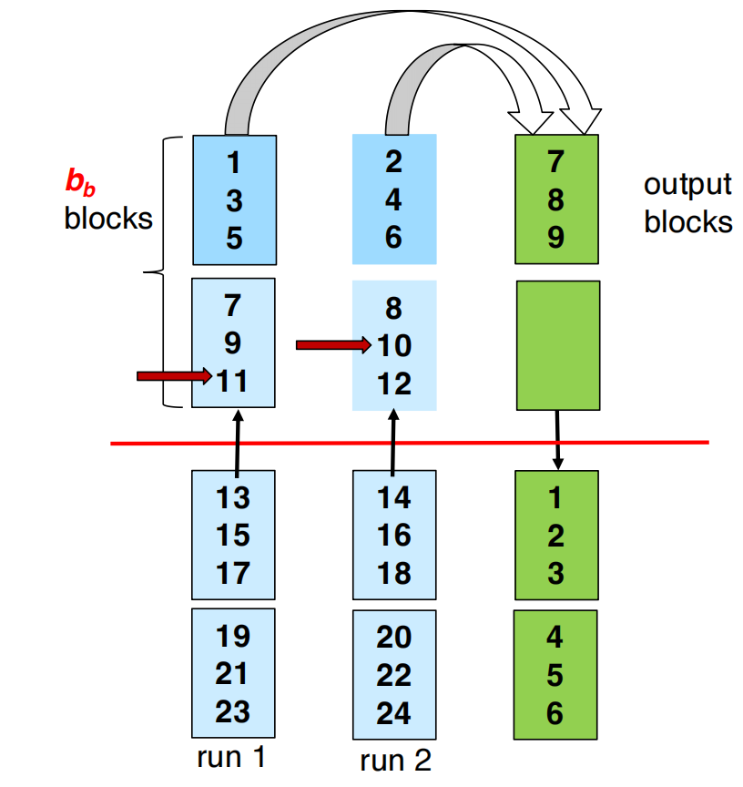
一轮可合并的 run 数变成:
这里的 -1 是因为要留一组 buffer 给 output。
merge pass 数:
block transfers 仍然是:
因为一次读 1 个 block 还是一次读 个 blocks,总共读写的数据量不变。
seek 数减少为:
假设:
b_r = 1000M = 100b_b = 5一次 merge 能合并:
初始 run 数仍是:
所以仍然只需要一轮 merge:
merge 阶段 seeks 约为:
比 simple version 的 1000 次 seeks 少很多。
代价是:每个 run 占用 5 个 buffer blocks,一次可合并的 runs 数从 99 降到 19。
NOTEadvanced version 的本质是:
用更多 buffer 换更少 seeks。
增大时,每次 seek 后能连续读写更多 blocks;但一轮能合并的 runs 变少,可能导致 merge pass 增加。
所以这里存在 trade-off。
Join Operation
join 是查询处理中最重要也最昂贵的操作之一。
常见 join 算法:
- Nested-loop join
- Block nested-loop join
- Indexed nested-loop join
- Merge join
- Hash join
选择哪一种,取决于:
- 是否有索引;
- 是否是 equi-join / natural join;
- 两个 relation 是否已排序;
- 可用内存大小;
- relation 的 block 数和 tuple 数;
- join attribute 是否是 key;
- 数据是否 skew。
下面的例子使用:
| relation | records | blocks |
|---|---|---|
student | 5000 | 100 |
takes | 10000 | 400 |
为了理解 join 算法,可以先记住一句话:
join 的代价主要来自“为了找匹配 tuple,需要反复读另一张表,还是能用排序 / hash / index 快速定位”。
Nested-Loop Join
计算 theta join:
最直接的算法是:
for each tuple t_r in r: for each tuple t_s in s: if (t_r, t_s) satisfies theta: output t_r concatenated with t_s其中:
- 是 outer relation;
- 是 inner relation。
特点:
- 不需要 index;
- 可用于任意 join condition;
- 会检查所有 tuple pairs,代价很高。
有两张小表:
student
| ID | name |
|---|---|
| 1 | Alice |
| 2 | Bob |
| 3 | Cindy |
takes
| ID | course |
|---|---|
| 1 | DB |
| 1 | Math |
| 2 | OS |
| 4 | AI |
执行:
student natural join takesnested-loop 的逻辑是:
Alice(ID=1) 和 takes 的 4 条记录逐一比较 -> 匹配 DB、MathBob(ID=2) 和 takes 的 4 条记录逐一比较 -> 匹配 OSCindy(ID=3) 和 takes 的 4 条记录逐一比较 -> 无匹配共比较:
次。
真实数据库里如果是 5000 条和 10000 条记录,就会变成 5000×10000 次 tuple comparison。
如果 buffer 最坏情况下只能放两个 relation 各一个 block,代价为:
公式含义:
- 读 outer relation 自身:;
- outer 中每一条 tuple 都要触发一次 inner relation 全表扫描:;
- 每次重新扫描 inner,近似一次 seek,共 次;
- 读 outer blocks 也估计 次 seeks。
如果较小 relation 能完全放入内存,应把它作为 inner relation。
此时代价可降到:
以 student ⋈ takes 为例。
如果 student 作为 outer relation:
block transfers,seeks 为:
如果 takes 作为 outer relation:
block transfers,seeks 为:
虽然 takes 作为 outer 的 tuple 数更多,但它让 inner relation 变成更小的 student,所以 block transfers 反而少。
如果较小的 student 能完全放进内存,总 block transfers 只有:
因为只需把 student 读入内存一次,再扫描 takes 一次。
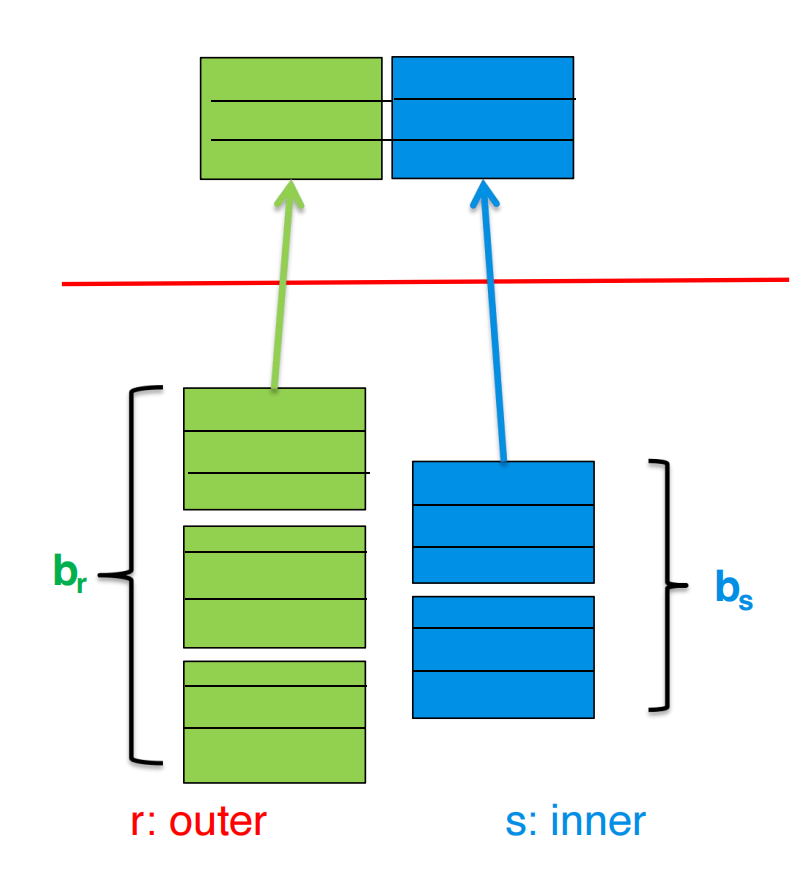
Block Nested-Loop Join
nested-loop join 按 tuple 配对,block nested-loop join 按 block 配对。
算法:
for each block B_r of r: for each block B_s of s: for each tuple t_r in B_r: for each tuple t_s in B_s: if (t_r, t_s) satisfies theta: output t_r concatenated with t_s核心变化:
普通 nested-loop 是 outer 每条 tuple 扫一遍 inner;block nested-loop 是 outer 每个 block 扫一遍 inner。
因此扫描 inner 的次数从 次降到 次。
最坏代价:
公式含义:
- outer 的每个 block 都要读一次,共 ;
- 对 outer 的每个 block,都完整扫描一次 inner,共 ;
- 每处理一个 outer block,约一次 outer seek 加一次 inner scan seek,所以 。
最好情况,如果 inner relation 保留在内存中:
继续使用:
student: 100 blockstakes: 400 blocks如果 student 是 outer,takes 是 inner:
相比普通 nested-loop 的:
差别非常大。
原因是一个 student block 里有很多 student tuples。block nested-loop 把这个 block 中的所有 tuples 一起和 takes 当前 block 比较,避免对每条 student tuple 都重新扫描 takes。
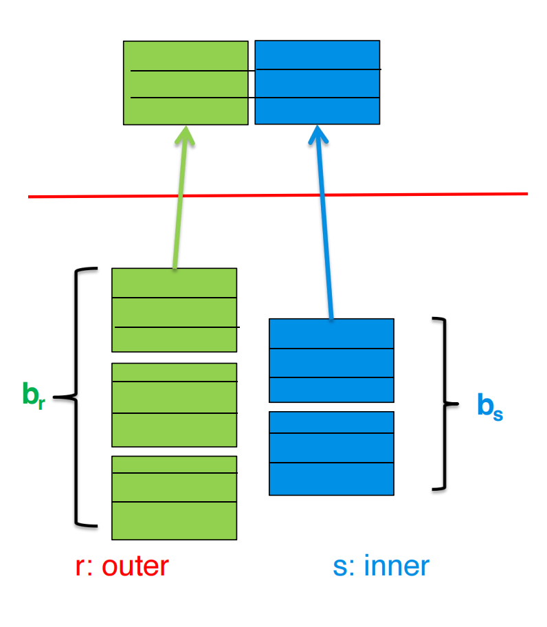
使用更多 buffer 的改进
如果内存有 个 blocks,可以把 outer relation 按 个 blocks 为单位读入。
剩下两个 blocks:
- 1 个给 inner relation;
- 1 个给 output。
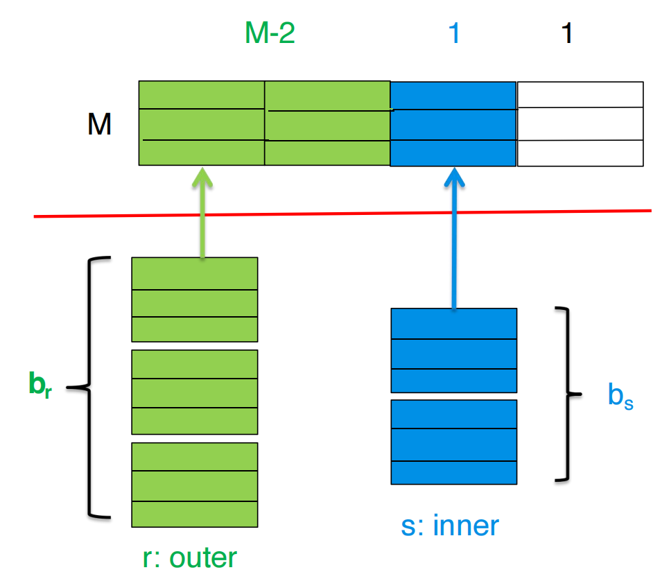
outer 被分成:
个 chunks。
每个 chunk 都要扫描一遍 inner relation。
代价:
设:
student: b_r = 100 blockstakes: b_s = 400 blocksM = 12 blocks每次可读入 outer 的:
个 blocks。
outer chunks 数:
所以只需要扫描 takes 10 次,而不是 100 次。
block transfers:
这比只用 1 个 outer block 的 40100 又少了一个数量级。
如果 outer relation 能放入内存,即:
则代价为:
其他优化:
- 如果 equi-join attribute 在 inner relation 中是 key,找到第一个匹配后即可停止 inner loop;
- inner relation 可正向、反向交替扫描,配合 LRU 保留部分 block,减少重复 I/O。
NOTE正向 / 反向交替扫描的意思是:
这样上一轮刚读到 buffer 里的尾部 blocks,下一轮可能还能继续使用,减少重新读盘。
Indexed Nested-Loop Join
如果满足:
- join 是 equi-join 或 natural join;
- inner relation 的 join attribute 上有 index;
则可以用 index lookup 替代 inner relation 的文件扫描。
算法:
for each tuple t_r in outer relation r: use index on s to find matching tuples in inner relation s output matches最坏情况中,outer relation 每个 tuple 都要做一次 index lookup。
代价:
其中 是对 inner relation 做一次 selection 的代价。
如果两个 relation 的 join attributes 上都有索引,通常选择 tuple 数较少的 relation 作为 outer relation。
小例子:
student
| ID | name |
|---|---|
| 1 | Alice |
| 2 | Bob |
| 3 | Cindy |
takes
| ID | course |
|---|---|
| 1 | DB |
| 1 | Math |
| 2 | OS |
| 4 | AI |
假设 takes.ID 上有 B+ 树索引:
ID=1 -> ptr(takes row 1), ptr(takes row 2)ID=2 -> ptr(takes row 3)ID=4 -> ptr(takes row 4)执行 student ⋈ takes 时:
Alice(ID=1): 用 takes.ID index 查 1 -> DB, MathBob(ID=2): 用 takes.ID index 查 2 -> OSCindy(ID=3): 用 takes.ID index 查 3 -> no match这里不再对每个 student 扫描整个 takes,只做一次 index lookup。
计算:
设 takes 在 ID 上有 primary B+-tree index,每个 index node 平均 20 个 entries。
takes 有 10000 tuples,因此 B+-tree 高度为 4,还需要 1 次访问 data block。
student 有 5000 tuples,存放在 100 blocks 中。
block nested-loop join 代价:
block transfers,seeks 为:
indexed nested-loop join 代价:
这里每个 student tuple 对 takes 做一次 index lookup,需要:
4 次 index block 访问 + 1 次 data block 访问 = 5所以是:
读 student 一次:1005000 个 student tuple 各查一次 takes index:5000 * 5WARNINGIndexed nested-loop join 不一定总是快。
如果 inner index 是 secondary index,而且每次 lookup 返回很多分散 records,那么 会很大。
例如
dept_name上的 secondary index,每个 department 有大量员工,查一次可能返回很多随机 data blocks。此时 indexed nested-loop 可能输给 block nested-loop 或 hash join。
Merge Join
merge join 也叫 sort-merge join。
适用于:
- equi-join;
- natural join。
基本步骤:
- 如果两个 relation 尚未按 join attribute 排序,先排序;
- 对两个有序 relation 做 merge;
- 对 join attribute 相同的 tuple 进行配对输出。
核心思想:
两边都按 join key 排序后,可以像归并排序一样用两个指针从前往后扫。
student 按 ID 排序:
ID=1 AliceID=2 BobID=4 CindyID=5 Davidtakes 按 ID 排序:
ID=1 DBID=1 MathID=3 OSID=4 AIID=5 DB做:
student join takes on student.ID = takes.ID用两个指针:
student.ID=1, takes.ID=1 -> 相等,输出 Alice-DB, Alice-Mathstudent.ID=2, takes.ID=3 -> 2 < 3,student 指针后移student.ID=4, takes.ID=3 -> 4 > 3,takes 指针后移student.ID=4, takes.ID=4 -> 相等,输出 Cindy-AIstudent.ID=5, takes.ID=5 -> 相等,输出 David-DB它不会反复扫描另一张表,每边基本顺序扫一遍。
关键区别:
普通 merge 只需要取较小值推进;merge join 遇到重复 join key 时,需要输出所有匹配组合。
如果:
r 中 ID=1 有 2 条:r1, r2s 中 ID=1 有 3 条:s1, s2, s3那么 join 结果必须输出:
r1-s1, r1-s2, r1-s3r2-s1, r2-s2, r2-s3一共:
条。
所以 merge join 需要处理重复 key 的 group,而不是简单跳过相等值。
如果两个 relation 已经按 join attribute 排好序,并且相同 key 的 tuple 能放进内存,则每个 block 只需读一次。
代价:
如果 relation 未排序,还要加上 sorting cost。
公式含义:
- :两个 relation 各顺序扫描一遍;
- :读 时,每次 seek 后连续读 blocks;
- :读 同理。
buffer 分配优化
设总 buffer memory 为 pages,分给 relation 的 buffer 数为 ,分给 relation 的 buffer 数为 。
约束:
估计代价:
其中前两项是 block transfers,后两项近似是 seeks。
为了最小化 seek,近似最优分配为:
直观理解:
block 数越多的 relation,应分到更多 buffer;但比例不是 ,而是 。
假设:
b_r = 100b_s = 400M = 30则:
buffer 分配比例:
r : s = 10 : 20 = 1 : 2所以:
不是按照 分。
原因是 buffer 的边际收益递减。给大表更多 buffer 是合理的,但不需要按表大小线性分配。
Hybrid Merge Join
如果:
- 一个 relation 已经按 join attribute 排序;
- 另一个 relation 在 join attribute 上有 secondary B+-tree index;
可以使用 hybrid merge join。
步骤:
- 将已排序 relation 与另一个 relation 的 B+-tree leaf entries 合并;
- 得到的结果中包含未排序 relation 的 tuple 地址;
- 按这些地址排序;
- 按物理地址顺序扫描未排序 relation,用真实 tuple 替换地址。
这样做的原因是:
按物理地址顺序扫描,比根据 index pointer 随机访问大量 tuple 更高效。
假设:
student已经按ID排序;takes没有按ID排序,但在takes.ID上有 secondary index。
直接 indexed nested-loop 会变成:
对每个 student.ID,到 takes.ID index 找 pointer再根据 pointer 随机访问 takes data blockshybrid merge join 的做法是:
1. 顺序扫描 student2. 顺序扫描 takes.ID 的 B+ tree leaves3. 先得到匹配的 takes record addresses4. 把这些 addresses 按磁盘物理位置排序5. 最后按物理顺序读取 takes records这样把很多随机访问转换成较顺序的访问。
Hash Join
hash join 适用于:
- equi-join;
- natural join。
它的核心思想是:
join key 相同的 tuple 经过同一个 hash function 后,一定落入同一个 partition。
设 join attributes 为 JoinAttrs,hash function 为 。
将 和 分区:
那么只需要比较:
不需要比较 和 ,其中 。
假设按 ID join,用 hash function:
那么:
ID=1 -> partition 1ID=2 -> partition 2ID=3 -> partition 0ID=4 -> partition 1如果 student.ID = takes.ID,它们的 ID 相同,所以一定进入同一个 partition。
因此:
student partition 1 只需要和 takes partition 1 比较student partition 2 只需要和 takes partition 2 比较student partition 0 只需要和 takes partition 0 比较这避免了全表两两比较。
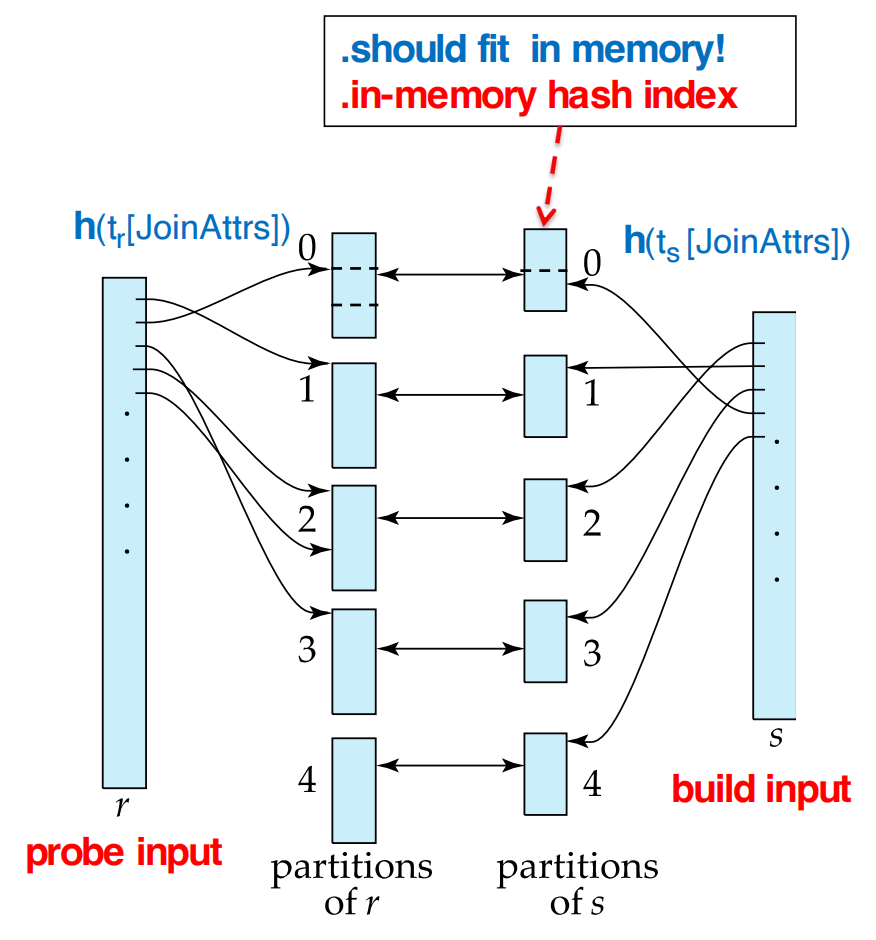
build input 和 probe input
通常选择较小的 relation 作为 build input。
- build input:先放入内存并建立 in-memory hash index;
- probe input:逐 tuple 读取,用来 probe 这个 hash index。
在 slides 中:
- 是 build input;
- 是 probe input。
要求:
每个 build partition 应能放入内存。
一般选择 partition 数 满足:
实际系统还会乘一个 fudge factor,例如 1.2,减少 overflow 风险。
假设 build input s 有 100 blocks,内存有 20 blocks。
至少需要把 s 分成:
个 partitions。
这样理想情况下每个 build partition 大约 20 blocks,可以放进内存。
hash join 算法
1. Partition build input s using hash function h.2. Partition probe input r using the same hash function h.3. For each partition i: load s_i into memory build an in-memory hash index on s_i using another hash function scan r_i tuple by tuple for each t_r in r_i: find matching t_s in s_i output t_r concatenated with t_s注意:
- partition hash function 和 in-memory hash index 的 hash function 通常不同;
- probe input partition 不需要放入内存;
- build input partition 需要放入内存。
以 student ⋈ takes 为例,假设 student 较小,作为 build input。
第一步分区:
student -> student_0, student_1, student_2takes -> takes_0, takes_1, takes_2第二步逐 partition join:
load student_0 into memory, build hash table on IDscan takes_0, for each tuple probe hash table
load student_1 into memory, build hash table on IDscan takes_1, for each tuple probe hash table
load student_2 into memory, build hash table on IDscan takes_2, for each tuple probe hash table由于相同 ID 一定在同编号 partition 中,takes_0 不需要和 student_1 或 student_2 比较。
Recursive Partitioning
如果 partition 数大于可用 buffer 数,就不能一次分成足够多 partitions。
这时需要 recursive partitioning:
- 先用 个 output buffers 分区;
- 对每个 partition 再用新的 hash function 继续分区;
- probe input 也必须使用相同的递归分区方式。
避免递归分区的大致条件是:
假设内存为 12MB,block size 为 4KB。
内存页数:
可以处理的 build relation 大小约为:
因此,内存看起来不大,但由于 hash join 分区后只需每个 build partition 放进内存,能处理远大于内存的数据。
NOTE为什么条件大致是 ?
一次最多能分出约 个 partitions。
如果 build relation 有 个 blocks,每个 partition 平均大小约为:
希望每个 partition 能放进内存:
所以:
即:
Partition Skew and Overflow
partitioning skew 指某些 partitions 明显比其他 partitions 大。
hash-table overflow 发生在:
某个 build partition 放不进内存。
常见原因:
- join attribute 上有大量重复值;
- hash function 分布不好;
- 数据本身 skew 严重。
如果很多 tuples 的 dept_name 都是 'Comp. Sci.',而 join key 正是 dept_name,那么无论 hash function 怎么设计,这些 'Comp. Sci.' tuples 都必须进入同一个 partition。
这个 partition 可能远大于其他 partitions,甚至放不进内存。
处理方法:
-
overflow resolution
- 在 build phase 发现 overflow 后,用另一个 hash function 继续划分 ;
- 对应的 也必须相同方式划分。
-
overflow avoidance
- 预先更谨慎地分区;
- 例如先分成更多 partitions,再把小 partitions 组合起来。
如果大量 tuple 拥有完全相同的 join key,上述方法都可能失败。
fallback:
对 overflowed partitions 使用 block nested-loop join。
Cost of Hash Join
如果不需要 recursive partitioning,hash join 的 block transfers 为:
其中:
- :分区阶段读入并写出两个 relation;
- :build/probe 阶段再次读入所有 partitions;
- :partially filled blocks 的额外开销。
NOTE为什么是 ?
hash join 有两个主要阶段。
第一阶段 partition:
第二阶段 build/probe:
加起来:
是因为每个 partition 的最后一个 block 可能没填满,但仍要写出和读回。
如果每个 input/output buffer 分配 blocks,则 seeks 为:
如果需要 recursive partitioning,设 partitioning passes 数:
则 block transfers:
seeks:
如果整个 build input 能放进内存,则不需要 partitioning,代价降为:
设:
M = 20 blocksb_instructor = 100b_teaches = 400选择 instructor 作为 build input。
将 instructor 分成 5 个 partitions,每个 20 blocks。
teaches 也分成 5 个 partitions,每个 80 blocks。
忽略 partially filled blocks,block transfers:
若 ,seeks:
Hybrid Hash Join
hybrid hash join 适合:
- memory 相对较大;
- build input 大于内存,但不是大很多。
核心优化:
build relation 的第一个 partition 直接留在内存中,不写回磁盘。
这样 probe relation 的第一个 partition 也可以直接 probe,不需要先写盘再读回。
设 memory size 为 25 blocks,instructor 分成 5 个 partitions,每个 20 blocks。
内存分配:
- 第一个 build partition 占 20 blocks;
- 1 个 block 用于 input;
- 另外 4 个 blocks 分别作为其余 4 个 partitions 的 output buffer。
teaches 也分成 5 个 partitions,每个 80 blocks。
第一个 teaches partition 直接用于 probe,不写出到磁盘。
plain hash join 代价:
hybrid hash join 代价:
因为第一个 build partition 20 blocks 和第一个 probe partition 80 blocks 避免了写出再读回。
NOTEhybrid hash join 的直观理解:
普通 hash join 会把所有 partitions 都写到磁盘,再读回来 join。
hybrid hash join 发现:既然内存够放一个 build partition,就不要把它写出去了。probe relation 中对应 partition 到来时,直接和内存中的 build partition join。
Complex Joins
conjunctive join condition
条件形式:
可以采用两种方式:
- 使用 nested-loop / block nested-loop,直接测试完整条件;
- 先用某个简单条件 计算 join,再在中间结果上检查剩余条件。
即:
然后过滤:
select *from r, swhere r.A = s.A and r.B > s.B;可以先对 r.A = s.A 使用 hash join 或 merge join,得到中间结果。
然后在中间结果中检查:
r.B > s.B这样可以利用 equi-join 算法处理其中一部分条件。
disjunctive join condition
条件形式:
可以:
- 直接用 nested-loop / block nested-loop;
- 分别计算每个简单 join,然后取 union:
where r.A = s.A or r.C = s.C可以分别计算:
r.A = s.A 的 joinr.C = s.C 的 join再把两个结果取 union。
要注意去重,因为同一对 tuple 可能同时满足两个条件。
Semijoin
semijoin 记作:
含义是:
输出 中那些至少能在 中找到一个匹配 tuple 的 tuple,但输出结果只包含 的属性。
如果某个 tuple 在 中出现 次,并且至少有一个 与它匹配,那么它在 semijoin 结果中也出现 次。
也就是说,semijoin 保留 中 tuple 的重复次数。
可以由普通 join 表达为:
但直接这样做可能产生很大的中间结果。
student ⋉ takes 表示:
找出至少选过一门课的学生。
如果用普通 join:
Alice 选了 DB 和 Math -> join 结果里 Alice 出现两次Bob 选了 OS -> Bob 出现一次然后再 projection 回 student 属性,还要去重。
semijoin 可以直接判断:
Alice 在 takes 中有匹配 -> 输出 Alice 一次Bob 在 takes 中有匹配 -> 输出 Bob 一次Cindy 无匹配 -> 不输出它避免了输出 student 与每门课拼接后的大结果。
更好的实现方式:
- block nested-loop semijoin:扫描 ,只要发现某个 tuple 有匹配就输出该 tuple,并可停止继续找该 tuple 的其他匹配;
- indexed nested-loop semijoin:对每个 tuple 在 的 index 中查是否存在匹配,存在就输出 tuple;
- merge semijoin:两个输入按 join key 排序,扫描时只输出左侧匹配 tuple;
- hash semijoin:对 建 hash table,对 probe,只要有匹配就输出 tuple。
NOTEsemijoin 和 join 的区别在输出。
- join 输出 和 拼接后的 tuple;
- semijoin 只输出 的 tuple;
- semijoin 常用于减少数据传输或减少后续操作输入规模。
Joins over Spatial Data
空间数据 join 的条件通常不是等值比较,而是:
- contains
- overlaps
- contained in
- nearest neighbor
- distance within a threshold
这类条件没有简单的一维排序关系,因此:
- merge join 通常不适用;
- hash join 也很难保证满足空间谓词的对象落入同一 hash bucket;
- nested-loop join 总能用,但大数据集上通常很慢。
更好的做法是使用 indexed nested-loop join,并利用空间索引:
- R-tree
- k-d tree
- k-d-B tree
- quadtree
这些索引支持快速检索重叠、包含、邻近等空间关系。
查询:
find all restaurants within 1km of each hotel这不是普通等值 join。
更合理的执行方式是:
for each hotel: use spatial index on restaurants find restaurants whose coordinates are within 1km这本质上是 indexed nested-loop join,只是 inner relation 上的索引不是 B+ 树,而是空间索引。
Other Operations
Duplicate Elimination
duplicate elimination 可以通过 sorting 或 hashing 实现。
sorting 方法
排序后,重复 tuple 会相邻出现。
然后只保留其中一份。
优化:
- 在 run generation 阶段就删除当前 run 内重复项;
- 在 intermediate merge 阶段继续删除重复项;
- 最终 run 中没有重复项。
hashing 方法
重复 tuple 会落入同一个 bucket。
构建 hash index 时:
- 如果 tuple 不存在,就插入;
- 如果 tuple 已存在,就丢弃。
最后输出 hash index 中的 tuple。
NOTESQL 默认保留重复项。
原因是 duplicate elimination 代价较高,所以 SQL 只有在显式使用
DISTINCT时才要求去重。
Projection
projection 的基本过程是:
- 对每个 tuple 取出 projection list 中的属性;
- 如果需要集合语义,再做 duplicate elimination。
如果 projection list 包含原 relation 的 key,则不会产生重复项,可以省去 duplicate elimination。
例如:
select ID, namefrom instructor;如果 ID 是 key,则不需要额外去重。
Aggregation
aggregation 与 duplicate elimination 类似,都需要把同组 tuple 放到一起。
可以使用:
- sorting:按 group-by attributes 排序;
- hashing:按 group-by attributes 分桶。
然后对每组应用 aggregate function。
select dept_name, avg(salary)from instructorgroup by dept_name;需要把相同 dept_name 的 tuples 聚在一起,再计算平均工资。
优化:partial aggregation。
在 run generation 或 intermediate merge 阶段就合并同组数据。
对不同 aggregate function:
| 聚合函数 | 可维护的中间状态 |
|---|---|
count | 当前计数 |
min | 当前最小值 |
max | 当前最大值 |
sum | 当前和 |
avg | sum 和 count,最后再相除 |
TIP
avg不适合直接合并平均值。应维护:
最后计算:
Set Operations
集合操作包括:
- union:
- intersection:
- difference:
可以通过两类方式实现:
- 先排序,再类似 merge join 同步扫描;
- 使用 hash join 的变体。
hashing 实现
第一步:用同一个 hash function 分区:
r -> r0, r1, ..., rns -> s0, s1, ..., sn然后逐 partition 处理。
union
对每个 partition :
- 对 建 in-memory hash index;
- 扫描 ,如果 tuple 不在 hash index 中,就加入;
- 扫描结束后输出 hash index 中所有 tuples。
intersection
对每个 partition :
- 对 建 in-memory hash index;
- 扫描 ;
- 如果 中 tuple 出现在 hash index 中,则输出。
difference
计算 。
对每个 partition :
- 对 建 in-memory hash index;
- 扫描 ;
- 如果 中 tuple 出现在 hash index 中,则从 index 删除;
- 最后输出 hash index 中剩余 tuples。
Outer Join
outer join 可以通过两种方式实现。
join 后补 null
以 left outer join 为例:
可以先计算普通 join:
然后找出没有参与 join 的 tuples:
再把这些 tuple 用 的属性补上 null,加入结果。
修改 join 算法
也可以直接修改 join 算法。
对于 merge join:
- 在 merging 过程中,如果某个 tuple 没有匹配 tuple;
- 直接输出该 tuple,并将 的属性填 null。
对于 hash join:
- 如果 是 probe relation,probe 时发现没有匹配,就输出 null-padded tuple;
- 如果 是 build relation,则 probe 时记录哪些 tuple 被匹配;最后输出未匹配的 tuple 并补 null。
right outer join 和 full outer join 可以类似处理。
Keyword Queries
关键词查询常用 inverted index。
形式:
keyword -> sorted list of document ids例如:
Silberschatz -> d1, d9, d21查询多个关键词:
K1, K2, ..., Kn做法:
- 分别取出每个关键词的 inverted list;
- 对这些有序列表做 intersection;
- 得到同时包含所有关键词的 documents。
如果允许返回至少包含 个关键词的文档,也可以修改 merge 过程。
真实搜索系统还会存储:
- term frequency
- inverse document frequency
- PageRank
- term positions
用于排序和 top-k retrieval。
Evaluation of Expressions
前面讨论的是单个关系代数操作。
但一个 SQL 查询通常会变成一棵 operator tree。
整体执行有两种基本策略:
- Materialization
- Pipelining
Materialization
materialized evaluation 的做法是:
从表达式树最低层开始,一次执行一个操作,并把中间结果写成临时关系。
然后上层操作再读取这些临时关系作为输入。
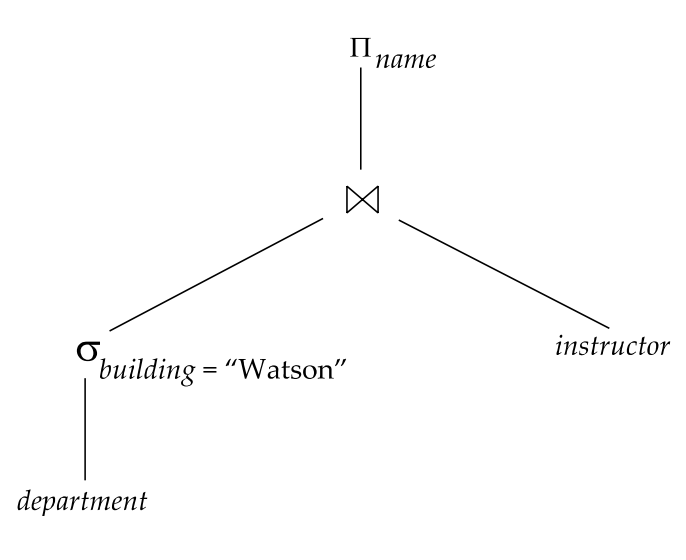
表达式:
materialization 的执行顺序:
- 先计算:
并把结果写入临时关系。
-
再计算它与
instructor的 join,并把结果写入临时关系。 -
最后做 projection:
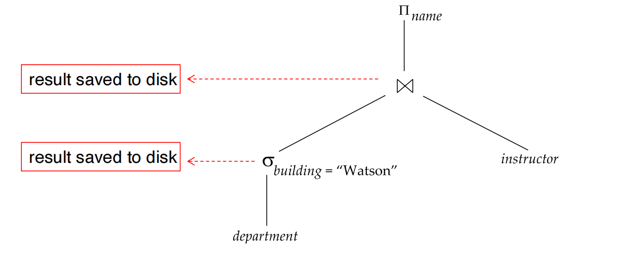
优点:
- 总是适用;
- 实现简单;
- 每个操作可以独立执行。
缺点:
- 中间结果写盘、读回的代价可能很高。
总代价应为:
sum of costs of individual operations+ cost of writing intermediate results+ cost of reading intermediate results前面单个操作的 cost formula 通常忽略中间结果写盘,所以做整体计划估计时必须额外加上。
Double Buffering
materialization 中可以使用 double buffering。
做法:
- 每个操作使用两个 output buffers;
- 一个 buffer 满了就写盘;
- 同时另一个 buffer 继续接收输出 tuple。
这样可以把磁盘写和计算部分重叠,减少总执行时间。
Pipelining
pipelined evaluation 的做法是:
多个操作同时执行,一个操作产生的 tuple 直接传给父操作,不写成临时关系。
对于前面的表达式:
- selection 产生的 tuple 直接送给 join;
- join 产生的 tuple 直接送给 projection;
- 不需要把中间结果写盘。
优点:
- 避免临时关系写盘;
- 可显著降低 I/O;
- 可更快产生第一批结果。
限制:
- 并非所有操作都能 pipeline;
- sort、hash join、merge join 等操作可能需要先读入大量输入才能输出结果;
- 这些操作称为 blocking operators。
Demand-Driven Pipelining
demand-driven 也叫 lazy evaluation 或 pull model。
执行方式:
- 顶层 operator 请求下一条 tuple;
- 它向子 operator 请求下一条 tuple;
- 子 operator 继续向自己的子 operator 请求;
- tuple 自底向上返回。
每个 operator 必须保存自己的 state。
例如 file scan 需要保存当前扫描到哪个 block、哪个 tuple。
特点:
- 父节点需要 tuple 时才向下拉取;
- 控制流从 root 往 leaf 传递请求;
- 数据流从 leaf 往 root 返回 tuple。
Producer-Driven Pipelining
producer-driven 也叫 eager evaluation 或 push model。
执行方式:
- 子 operator 主动产生 tuple;
- tuple 被写入父子 operator 之间的 buffer;
- 父 operator 从 buffer 中取 tuple。
如果 buffer 满了:
- child operator 暂停;
- 等 parent 消费 buffer 后继续产生。
系统调度那些:
- output buffer 有空间;
- input 已准备好;
- 可以继续处理的 operators。
Iterator Model
demand-driven pipelining 常用 iterator model 实现。
每个 operator 实现三个接口:
open()next()close()open
初始化 operator。
例如:
- file scan:把文件指针置到文件开始位置;
- merge join:先排序输入,并把两个输入指针置到开头。
next
返回下一条输出 tuple,并更新内部 state。
例如:
- file scan:输出当前 tuple,然后指针前移;
- merge join:从上次保存的状态继续 merge,直到找到下一条输出 tuple。
close
释放资源。
TIPiterator model 的关键是 state。
每次
next()返回后,operator 必须知道下一次从哪里继续。
Blocking Operators
有些算法不能一边读输入一边输出完整结果。
典型 blocking operators:
- sort:必须看到足够多输入后才能输出全局有序结果;
- hash join:通常需要先构建 build input 的 hash table;
- merge join:如果输入还没排序,需要先排序。
因此 pipeline 中常常会出现 blocking edge。
一些算法变体可以输出部分结果:
- hybrid hash join:partition 0 留在内存中,probe relation 的 partition 0 读入时可以立即产生结果;
- double-pipelined hash join:同时缓存两个 relation 的 partition 0,新 tuple 到来时与另一侧已有 tuple 匹配并输出。
Continuous Stream Data
pipeline 也适用于 continuous-stream data。
流数据的特点是:
- 数据持续到达;
- 输入理论上没有终点;
- 不可能先 materialize 全部输入再处理。
因此 stream processing 更依赖 pipeline。
Query Processing in Memory
前面的分析主要围绕磁盘 I/O。
当数据已经在内存中时,主要瓶颈变成:
- CPU cost;
- cache miss;
- tuple interpretation overhead;
- memory bandwidth。
Cache-Conscious Algorithms
目标:
减少 cache misses,充分利用每次读入 cache line 的数据。
sorting
排序时,可以让初始 runs 大小接近 L3 cache。
这样 run 内排序期间,大部分数据留在 cache 中,减少 cache misses。
之后仍然按 merge-sort 思路合并。
hash join
hash join 可以两层分区:
- 第一层:让 build partition + probe partition 能放入 memory;
- 第二层:继续 subpartition,使 build subpartition + in-memory hash index 能放入 L3 cache。
这样 probe 阶段访问 hash table 时 cache miss 更少。
tuple layout
属性布局也会影响 cache。
原则:
经常一起访问的 attributes 应尽量相邻存放。
这能提高 cache line 利用率。
multithreading
使用多线程可以隐藏部分 cache miss stall。
当一个线程因 cache miss 停顿时,其他线程仍然可以继续执行。
Query Compilation
传统数据库执行引擎通常解释执行 query plan。
解释执行有开销:
- 每处理一条 tuple,都要根据 metadata 找 attribute 位置;
- 表达式计算需要通用解释器;
- 函数调用和分支判断较多。
query compilation 的思想是:
把 query plan 编译成机器码或中间代码,减少解释执行开销。
常见方式:
- 生成 Java bytecode;
- 生成 LLVM IR;
- JIT compilation。
适合场景:
- 内存数据库;
- OLAP 查询;
- 重复执行或处理大量 tuple 的查询。
Column-Oriented Storage
column-oriented storage 对查询处理也很重要。
如果查询只访问少数属性,列存可以避免读取无关列。
并且列存天然适合:
- vectorized execution;
- SIMD;
- query compilation;
- compression。
例如:
select avg(salary)from instructorwhere dept_name = 'Music';如果使用列存,系统主要读取:
dept_name columnsalary column不必读取整行中的其他属性。
NOTE行存适合一次访问整条记录的 OLTP;列存适合扫描大量记录但只访问少量列的 OLAP。
Query processing in memory 中,列存和 compilation、vectorized execution 常一起发挥作用。