

概述
这一章的核心是:
索引(index)是数据库为了加速数据访问而维护的辅助数据结构。它用额外空间和维护代价,换取更低的查询 I/O 成本。
索引最像图书馆的作者目录:
- 目录本身不保存完整书籍内容
- 目录按照某个查找键组织
- 通过目录可以快速定位目标记录的位置
数据库索引的基本权衡:
- Access time:查找是否更快
- Insertion time:插入是否更慢
- Deletion time:删除是否更慢
- Space overhead:额外占用多少空间
这一章的主线是:
- 先理解有序索引:primary / secondary、dense / sparse、multilevel index
- 再理解最重要的索引结构:B+-tree
- 再比较 B+-tree file organization 与 B-tree
- 再讨论多属性索引、主存索引、Flash 索引
- 最后理解写优化索引:LSM-tree、buffer tree,以及 bitmap index
目录
- 概述
- 目录
- Basic Concepts
- Ordered Indices
- Dense Index 与 Sparse Index
- Multilevel Index
- B+-Tree Index
- B+-Tree Example
- B+-Tree File Organization
- B-Tree Index Files
- Secondary Index 的记录移动问题
- Variable Length Keys 与 Prefix Compression
- Indices on Multiple Keys
- Indexing in Main Memory
- Bulk Loading and Bottom-Up Build
- Indexing on Flash
- Write Optimized Indices
- Bitmap Indices
Basic Concepts
索引机制用于加速对目标数据的访问。
一个索引文件通常比原始数据文件小得多,因为它保存的不是完整记录,而是:
search-key pointer其中:
search-key用于查找pointer指向数据记录、数据块,或者记录所在的 bucket
Search Key
Search key(搜索键) 是用于查找文件中记录的属性或属性集合。
search key 不一定是 primary key。
例如:
- 按
ID查 instructor,ID是 search key - 按
salary查 instructor,salary也是 search key - 按
(dept_name, salary)查 instructor,二者组成 composite search key
Index Entry
索引文件由很多 index entries 组成。
每个 index entry 的形式是:
(search-key value, pointer)这个 pointer 可以指向:
- 一条记录
- 一个数据块
- 一组拥有相同 search-key 的记录 bucket
- B+-tree 的子节点
TIP索引的本质不是“复制一份表”。
索引只保存能帮助定位数据的最小信息。
所以它通常比原始 relation 小很多。
两类基本索引
- Ordered Index
搜索键值按照排序顺序存储。
适合:
- 点查询
- 范围查询
- 按序扫描
- Hash Index
搜索键值通过 hash function 均匀分配到 bucket 中。
适合:
- 等值查询
不擅长:
- 范围查询
- 顺序扫描
这一章主要讨论 ordered index,尤其是 B+-tree。
评价一个索引的标准
设计索引时不能只看查询速度。
需要同时考虑:
- 支持的访问类型
- point query:查某个具体值
- range query:查某个范围内的值
- Access time
- Insertion time
- Deletion time
- Space overhead
索引加速查询,但会拖慢更新,并占用额外空间。
Ordered Indices
有序索引中,index entry 按 search-key value 排序。
典型例子:图书馆的作者目录。
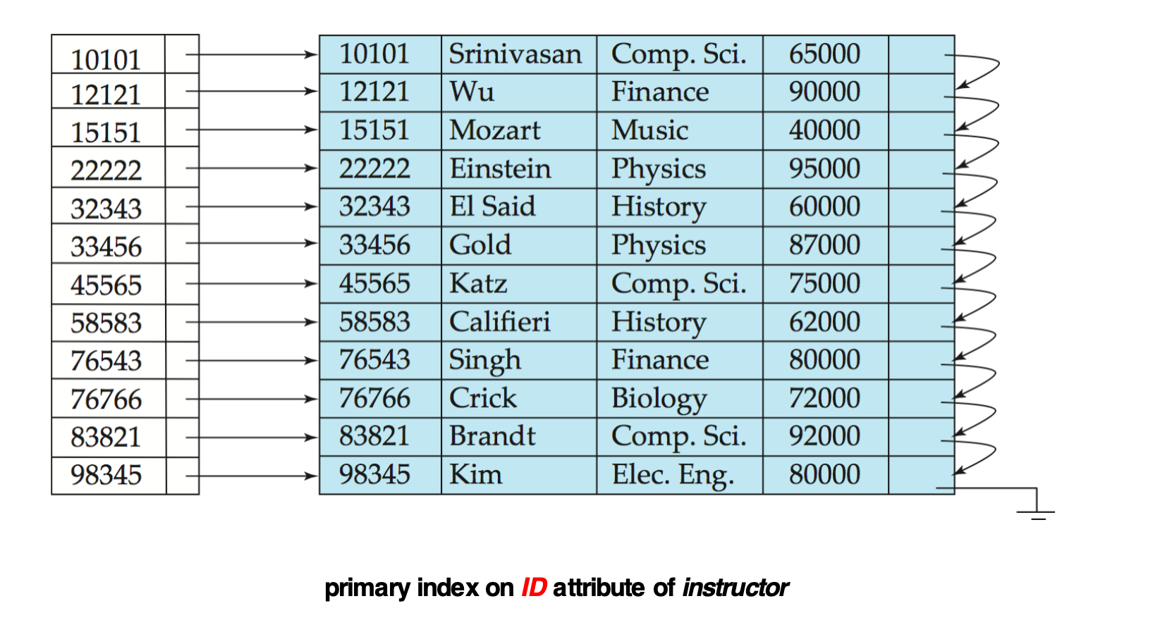
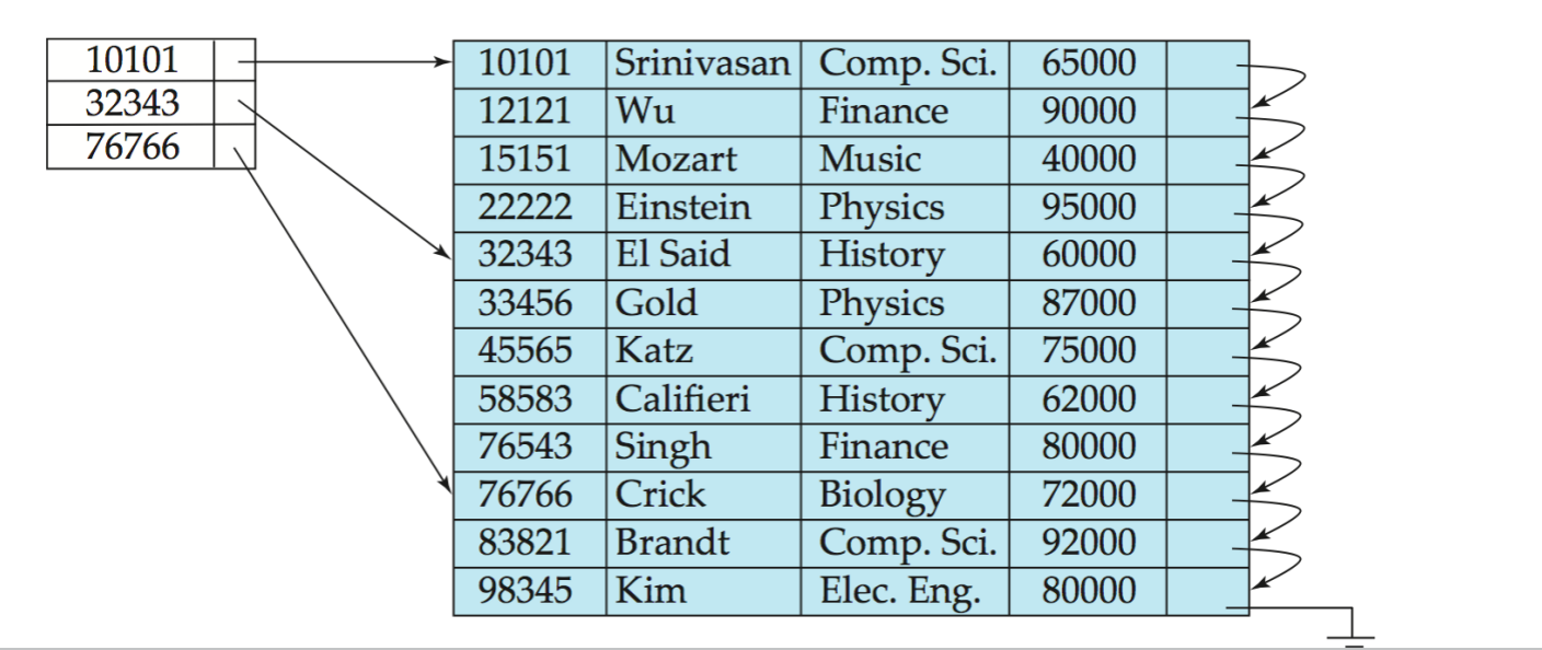
Primary Index / Clustering Index
Primary index 是建立在顺序文件上的索引,并且它的 search key 决定了数据文件本身的顺序。
它也叫:
- Clustering index(聚集索引)
例如:
instructor文件按照ID排序存储- 在
ID上建立的索引就是 primary index
WARNINGprimary index 的 search key 通常是 primary key,但不一定必须是 primary key。
这里的 primary 主要强调:
数据文件的物理顺序由这个 search key 决定。
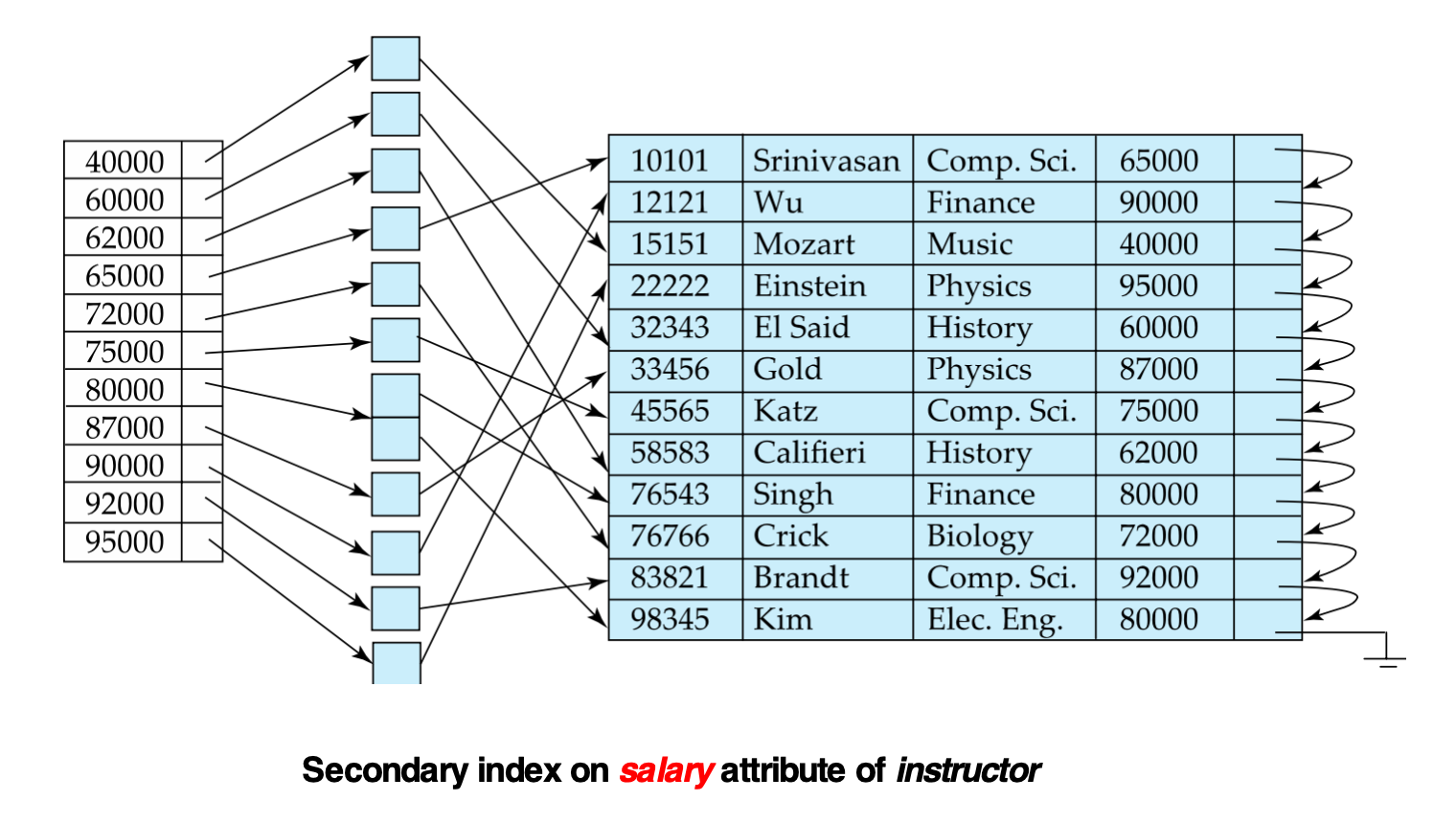
Secondary Index / Non-clustering Index
Secondary index 的 search key 顺序和数据文件的顺序不同。
它也叫:
- Non-clustering index(非聚集索引)
例如:
instructor文件按照ID排序存储- 但在
salary上建立索引 - 这个索引就是 secondary index
secondary index 的问题是:
- 相邻的索引项不一定对应相邻的数据记录
- 通过索引找到多个记录时,可能产生大量随机 I/O
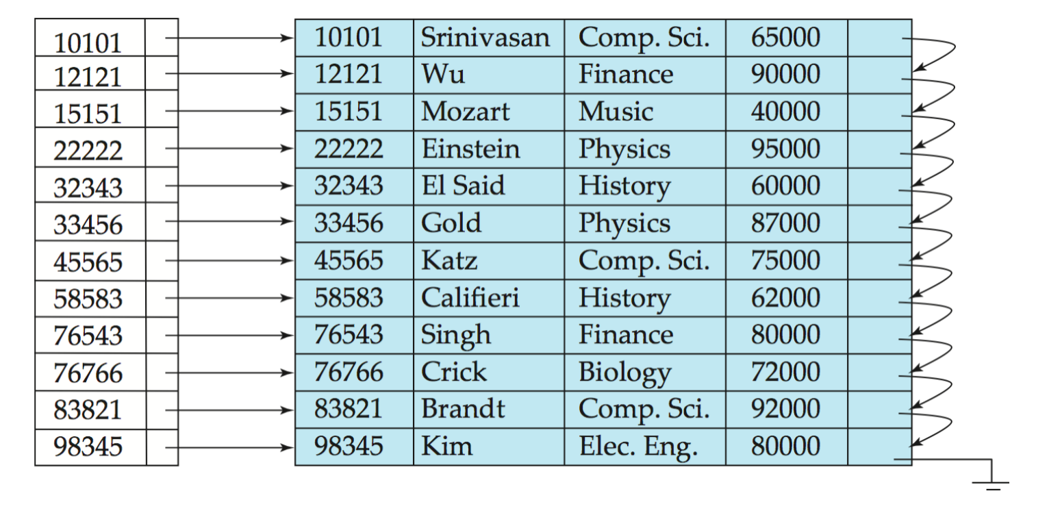
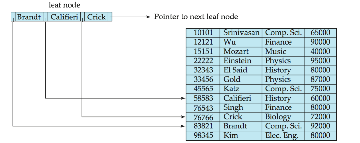
Index-Sequential File
**Index-sequential file(索引顺序文件)**是:
带有 primary index 的顺序文件。
它的基本思想是:
- 数据文件本身按 search key 排序
- 索引帮助快速定位文件中的位置
- 定位后可以顺序扫描
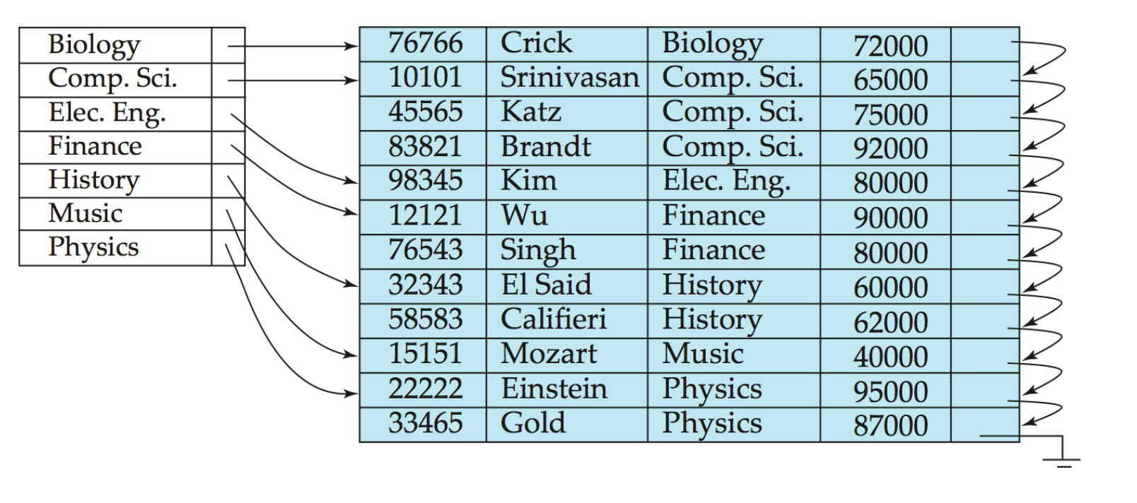
Dense Index 与 Sparse Index
Dense Index
**Dense index(稠密索引)**中,每个 search-key value 都有一个 index record。
如果 search key 是唯一的:
每条记录一个索引项如果 search key 不是唯一的:
每个不同的 search-key value 一个索引项索引项再指向一组记录例如:
- 在
instructor.ID上建立 dense index - 每个 instructor 的 ID 都出现在索引中
另一个例子:
- 文件按
dept_name排序 - 在
dept_name上建立 dense index - 每个不同的
dept_name有一个索引项
Sparse Index
**Sparse index(稀疏索引)**只为部分 search-key values 建立 index records。
它适用的前提是:
数据记录必须按照 search key 顺序排列。
查找 search-key value 为 K 的记录时:
- 在 sparse index 中找到最大且小于等于
K的 search-key value - 从该索引项指向的位置开始,在数据文件中顺序扫描
- 找到目标记录,或者发现目标不存在
Dense 与 Sparse 的对比
Dense index:
- 查找更快
- 占空间更多
- 插入删除维护成本更高
Sparse index:
- 占空间更少
- 插入删除维护成本更低
- 查找通常稍慢,因为需要从索引定位点开始顺序扫描
一个常用折中:
每个数据块建立一个 sparse index entry,记录该块中的最小 search-key value。
这样:
- 索引项数量约等于数据块数量
- 查找最多只需在一个块内继续扫描
- 空间和查找速度之间比较平衡
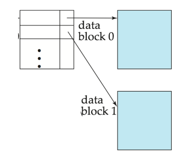
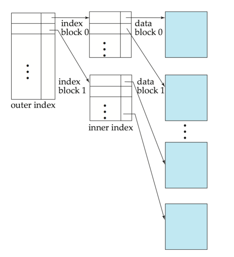
Multilevel Index
当 primary index 本身太大,不能放入内存时,每次查索引也会产生较高 I/O 成本。
解决办法:
把磁盘上的 primary index 当作一个顺序文件,再在它上面建立 sparse index。
于是形成两层:
- Inner index:原来的 primary index file
- Outer index:建立在 inner index 上的 sparse index
如果 outer index 仍然太大,还可以继续往上加层。
这就是 multilevel index(多级索引)。
WARNING多级索引提高查询效率,但更新更复杂。
当数据文件插入或删除记录时,所有受影响层级的索引都可能要更新。
B+-Tree Index
为什么需要 B+-Tree
传统 index-sequential file 的问题是:
- 文件不断增长后,会产生很多 overflow blocks
- 查询性能逐渐下降
- 需要周期性重组整个文件
B+-tree 的优势是:
- 插入、删除时只做局部调整
- 不需要周期性重组整个文件
- 树高很小,查询 I/O 次数少
- 实际数据库系统中使用非常广泛
代价是:
- 插入和删除逻辑更复杂
- 节点分裂、合并带来额外维护成本
- 有一定空间开销
B+-Tree 的结构约束
设一个 B+-tree 节点最多有 n 个 child pointers。
B+-tree 是一棵满足以下性质的有根树:
-
从 root 到所有 leaf 的路径长度相同
-
非 root、非 leaf 的 internal node 有个 children。
-
Leaf node 有个 search-key values。
-
特殊情况:
- 如果 root 不是 leaf,root 至少有 2 个 children
- 如果 root 是 leaf,root 可以有 0 到
n-1个 values
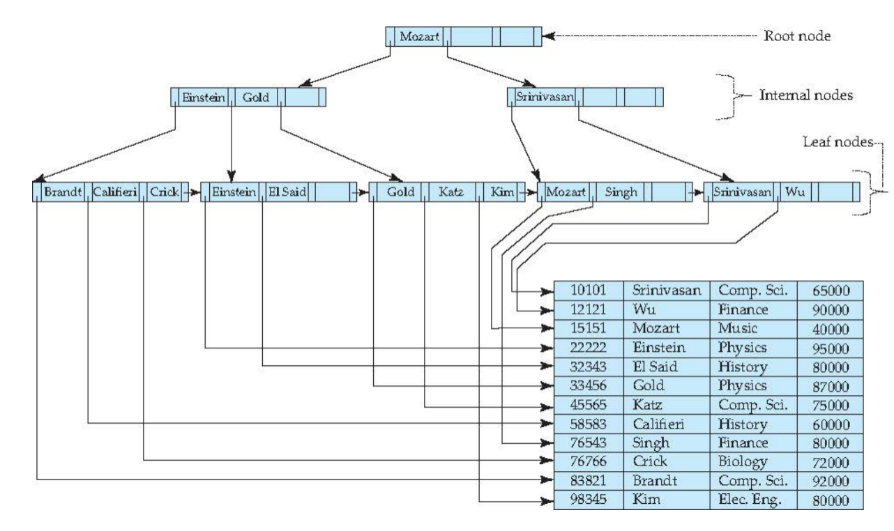
B+-Tree 节点结构
一个典型节点包含:
P1 K1 P2 K2 ... Pn-1 Kn-1 Pn其中:
Ki是 search-key valuesPi是 pointers- 在 non-leaf node 中,
Pi指向子节点 - 在 leaf node 中,
Pi指向记录或记录 bucket
- 在 non-leaf node 中,
节点内 search-key 按升序排列:
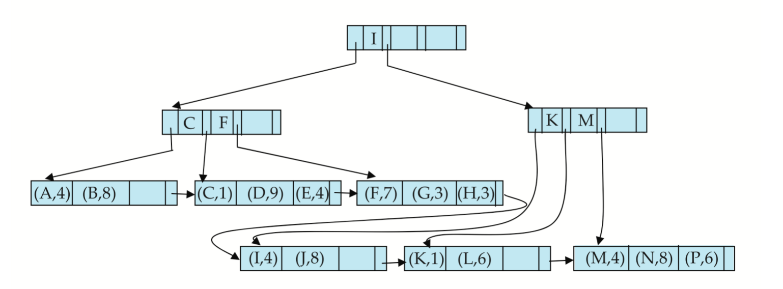
Leaf Node
Leaf node 保存真正用于定位记录的 entry。
对 leaf node:
- 对于
i = 1, 2, ..., n-1,Pi指向 search-key value 为Ki的记录或 bucket - 如果
Li和Lj是两个 leaf node,且i < j,则Li中的 key 都小于等于Lj中的 key Pn指向 search-key 顺序中的下一个 leaf node
最后一点很关键。
因为 leaf node 之间有链表连接,所以 B+-tree 很适合做范围查询:
- 先从 root 查到范围起点所在的 leaf
- 再沿着 leaf-level linked list 顺序扫描
Non-leaf Node
Non-leaf nodes 组成 leaf nodes 上方的多级稀疏索引。
对于一个有 m 个 pointers 的 non-leaf node:
P1指向的子树中所有 key 都小于K1Pi指向的子树中所有 key 满足:
Pm指向的子树中所有 key 都大于等于K_{m-1}
因此 non-leaf node 不直接保存完整数据记录,只负责导航。
Observations about B+ Tree
B+ 树的节点之间通过 pointer 连接,逻辑上相邻的节点不要求在磁盘上物理相邻。
例如,某个父节点可以指向任意位置的子节点;叶节点之间也可以通过指针连成有序链表。
这使得插入和删除时不需要大规模移动磁盘块,只需要修改局部节点和指针。
这也意味着:
- 逻辑相邻的叶节点可能分布在磁盘不同位置
- 范围查询虽然可以沿叶节点链表顺序扫描,但物理 I/O 未必完全连续
B+ 树的非叶节点可以看成是对下一层节点的索引,更准确地说是多级稀疏索引。
叶节点保存完整的搜索键以及指向记录的指针;非叶节点只保存部分 search-key,用来指导查询进入哪个子树。
若一个 B+ 树节点最多有 个子指针,则除根节点外:
- 非叶节点至少有 个子指针
- 叶节点至少有 个 search-key
- 如果根节点不是叶节点,根节点至少有 2 个子指针
因此,B+ 树每增加一层,能够覆盖的搜索键数量都会乘上一个较大的 fan-out。
如果文件中有 个 search-key,那么树高最多约为:
考虑根节点至少有 2 个孩子,也可近似写成:
所以 B+ 树的高度是对数级的:
实际数据库中,一个节点通常对应一个磁盘页,fan-out 往往很大,例如几十到上百。
因此即使有百万级记录,B+ 树也通常只有很少几层。
B+ 树的查找过程是:root -> internal node -> ... -> leaf node -> record。
每访问一层,就通过 search-key 缩小一次搜索范围。
所以查找代价与树高成正比。
插入和删除也只会沿着从根到叶的一条路径进行局部调整:
- 插入时,如果叶节点满了,分裂节点,并可能向父节点传播
- 删除时,如果节点太空,可以向兄弟节点借 entry,或者和兄弟节点合并
- 最坏情况下,调整传播到根
因此 B+ 树的查找、插入、删除都可以在对数时间内完成。
B+-Tree 查询
查找 search-key value V 的基本过程:
function find(V): C = root while C is not a leaf node: 找到最小的 i,使得 V <= Ki if 不存在这样的 i: C = C 中最后一个非空指针指向的子节点 else: if V == Ki: C = Pi+1 指向的子节点 else: C = Pi 指向的子节点
在 leaf node 中查找 Ki == V if 找到: 沿着对应 pointer 访问记录 else: 记录不存在这里 V == Ki 时走 Pi+1,是因为 non-leaf node 中的 Ki 是右侧子树的分界值。
B+-Tree 高度与 I/O 成本
B+-tree 的效率来自高 fanout。
如果有 K 个 search-key values,节点最大 fanout 为 n,则树高至多约为:
实际中:
- 一个节点通常等于一个磁盘块
- 磁盘块常见大小是 4KB
- 如果每个 index entry 约 40 bytes,
n大约为 100
例子:
K = 1,000,000n = 100- 最少 fanout 约为 50
查找最多访问:
个节点。
对比平衡二叉树:
如果每个节点访问都可能是一次磁盘 I/O,这个差距非常大。
TIPB+-tree 牺牲的是节点内部的线性 / 二分查找成本,换来的是极高 fanout。
数据库索引首先要减少磁盘 I/O 次数,所以高 fanout 很重要。
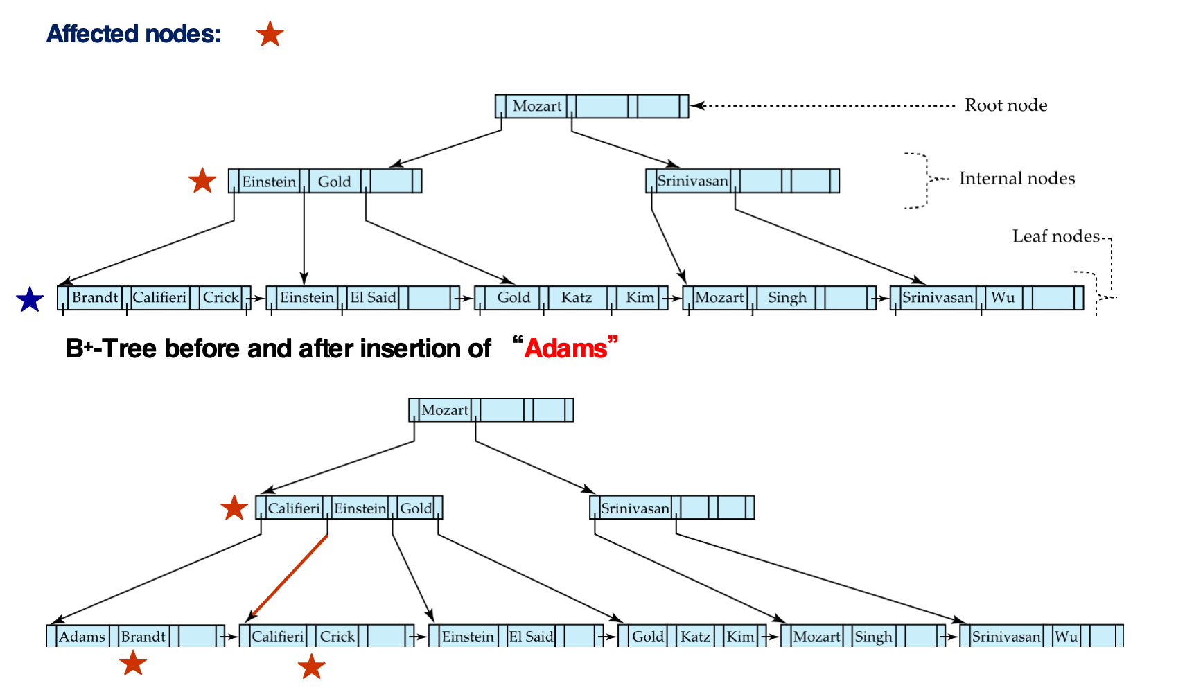
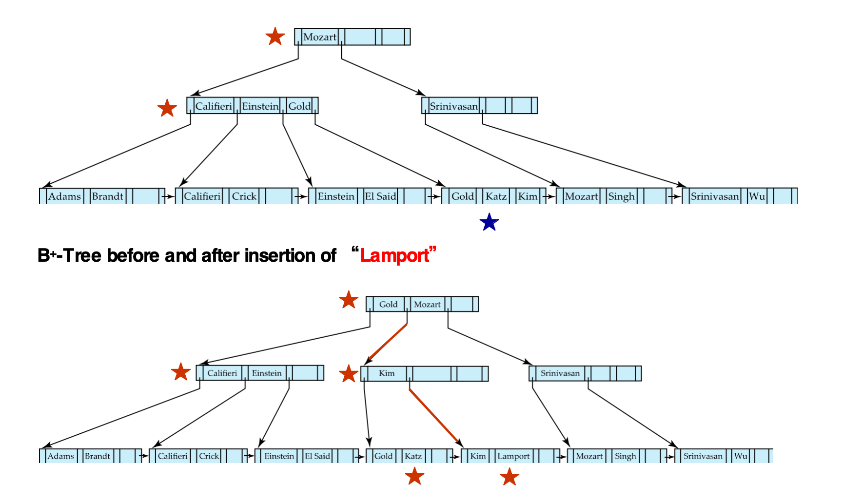
B+-Tree 插入
插入 (v, pr) 时,假设记录已经加入数据文件。
其中:
v是新记录的 search-key valuepr是指向该记录的 pointer
过程:
- 找到
v应该出现的 leaf node - 如果 leaf node 有空间,直接插入
(v, pr) - 如果 leaf node 已满,需要分裂 leaf node,并向父节点插入新的分隔项
Leaf node split 的规则:
- 把原节点中的 entries 加上新 entry,一共
n个(key, pointer),按 key 排序 - 前
ceil(n/2)个留在原 leaf - 剩下的放入新 leaf
- 设新 leaf 为
p,新 leaf 中最小 key 为k - 向父节点插入
(k, p) - 如果父节点也满,则继续向上分裂
- 最坏情况下 root 分裂,树高加 1
伪代码:
function insert(pr, v) // pr: pointer to the record // v : search-key value
L = find_leaf(v)
if L has space then insert (v, pr) into L in sorted order else split_leaf(L, v, pr)
function split_leaf(L, v, pr) T = all entries in L plus (v, pr), sorted by search key
keep first ceil(n / 2) entries in L create new leaf node L2 put remaining entries into L2
L2.next = L.next L.next = L2
k = smallest search-key value in L2
insert_in_parent(L, k, L2)
function insert_in_parent(N, k, N2) // insert separator key k and pointer N2 after node N
if N is root then create new root R R.keys = [k] R.pointers = [N, N2] root = R return
P = parent(N)
if P has space then insert (k, N2) into P after pointer to N else split_internal(P, k, N2)
function split_internal(P, k, N2) T = all keys and pointers in P plus (k, N2), in sorted order
split T into: left internal node P middle key k_mid right internal node P2
keep left part in P put right part in P2
insert_in_parent(P, k_mid, P2)插入 Adams:
Adams应插入最左边 leaf- 原 leaf 已满后发生 split
- 新 leaf 的最小 key 是
Califieri - 因此向 parent 插入
(Califieri, pointer-to-new-node)
插入 Lamport:
- 先插入到对应 leaf
- 如果 leaf split 后 parent 也满,split 会继续向上传播
- 这个例子展示了从 leaf 到 internal node 的级联调整
B+-Tree 删除
删除 (v, pr) 时,假设数据文件中的记录已经删除。
基本过程:
- 从 leaf node 中删除
(v, pr) - 如果 leaf node 仍满足最小 entry 数要求,结束
- 如果 leaf node underfull,分两种情况处理:
情况一:可以和 sibling 合并
如果当前节点和某个 sibling 的 entries 总数能放进一个节点:
- 把两个节点内容合并到一个节点中
- 删除另一个节点
- 在父节点中删除指向被删节点的 pointer 及对应分隔 key
- 父节点可能继续 underfull,因此递归处理
情况二:不能合并,只能重新分配
如果当前节点和 sibling 的 entries 总数放不进一个节点:
- 在当前节点和 sibling 之间重新分配 entries
- 让两个节点都满足最低占用要求
- 更新父节点中对应的 search-key value
如果 root 删除后只剩一个 child:
- 删除 root
- 唯一 child 成为新的 root
- 树高减 1
伪代码:
function delete(pr, v) // pr: pointer to the record // v : search-key value
L = find_leaf(v)
remove (v, pr) from L
if L is root then if L is empty then root = null return
if L has at least minimum number of entries then update parent separator keys if needed return
handle_underflow(L)
function handle_underflow(N) S = an adjacent sibling of N P = parent(N)
if entries of N and S fit in one node then merge N and S into one node delete corresponding separator key and pointer from P
if P is root and P has only one child then root = the only child of P return
if P has too few pointers then handle_underflow(P)
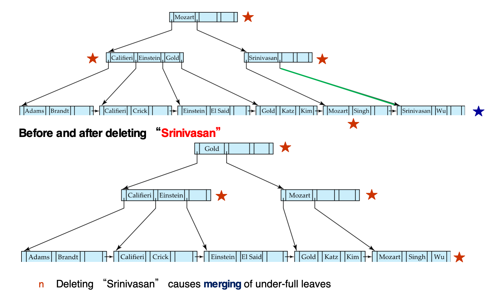
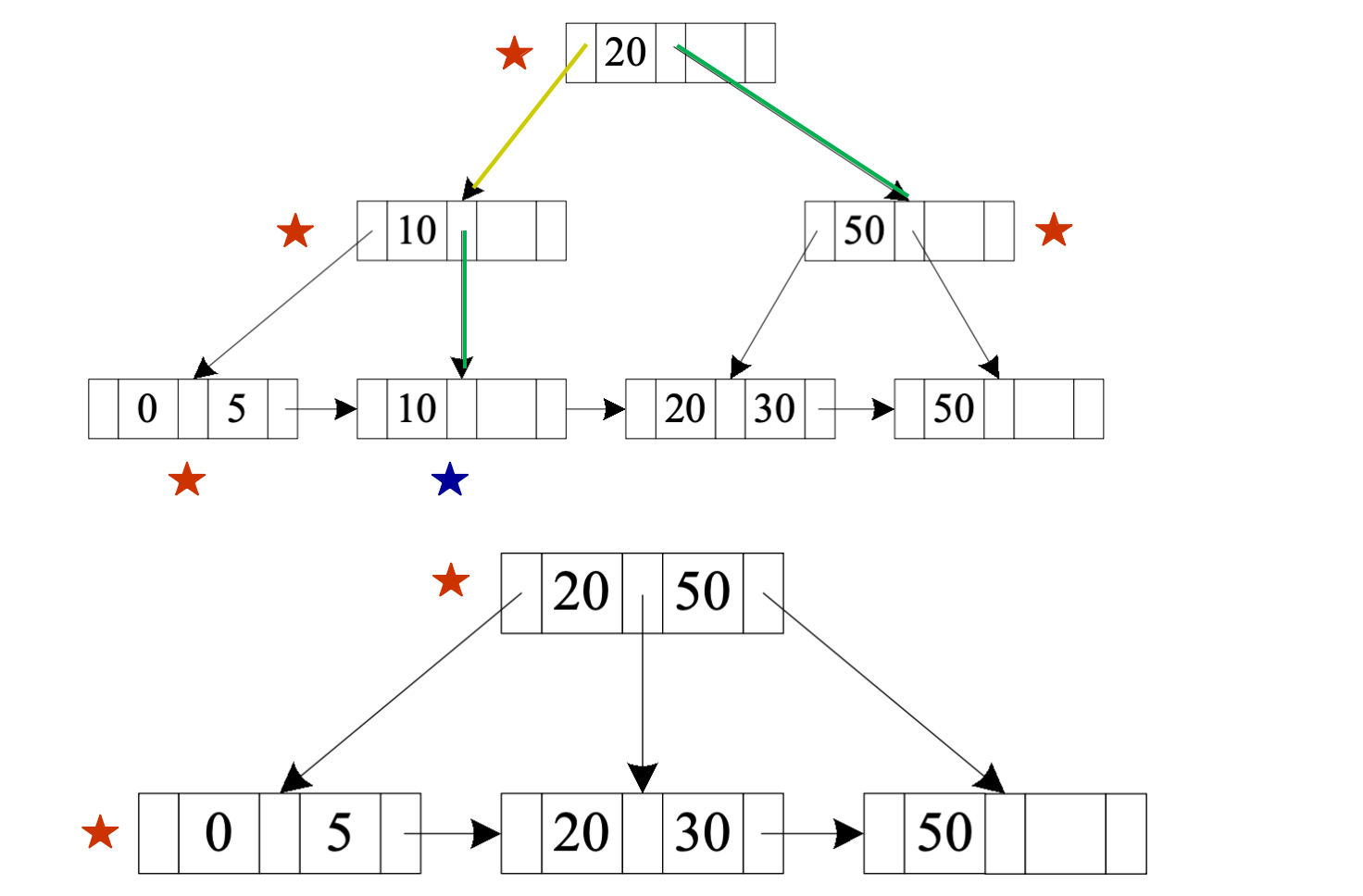
else redistribute entries between N and S update corresponding separator key in P删除 Srinivasan:
- 对应 leaf 删除后 underfull
- underfull leaf 与 sibling 合并
- parent 中相应指针和分隔 key 被删除
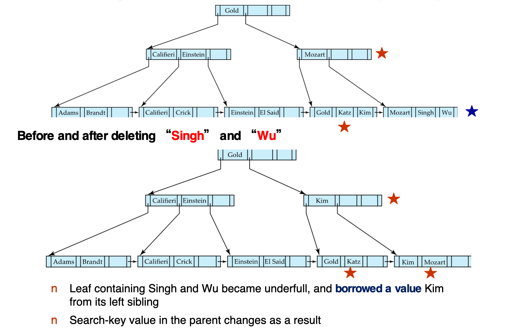
删除 Singh 和 Wu:
- 包含
Singh、Wu的 leaf 删除后 underfull - 它从左侧 sibling 借入
Kim - 因为 leaf 的最小 key 发生变化,parent 中对应 search-key value 也要更新
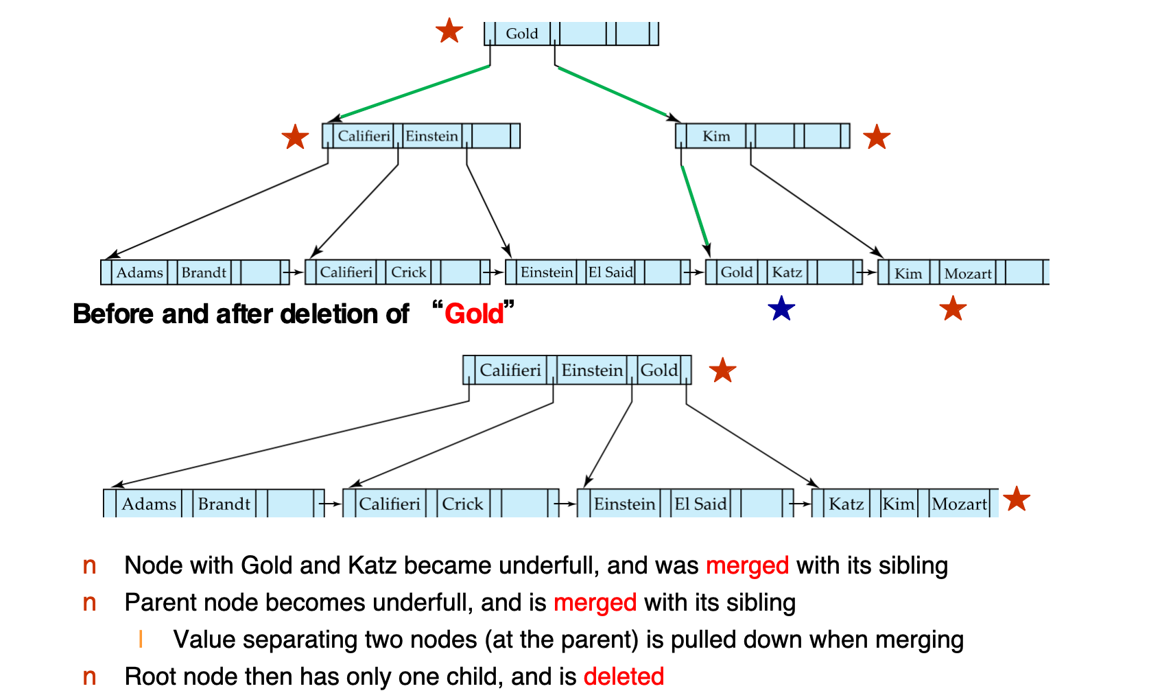
删除 Gold:
- 包含
Gold和Katz的节点 underfull - 该节点与 sibling 合并
- parent 也 underfull,继续与 sibling 合并
- 合并 internal node 时,parent 中用于分隔两个节点的 key 会被拉下来
- root 最后只剩一个 child,因此 root 被删除
插入删除代价与节点利用率
单个 entry 的插入 / 删除 I/O 成本与树高成正比。
如果有 K 个 entries,最大 fanout 为 n,则最坏复杂度是:
实际代价通常更低:
- internal nodes 往往缓存在 buffer 中
- split / merge 不常发生
- 大多数插入删除只影响 leaf node
平均节点占用率和插入顺序有关:
- 随机插入:约
2/3 - 按排序顺序插入:约
1/2
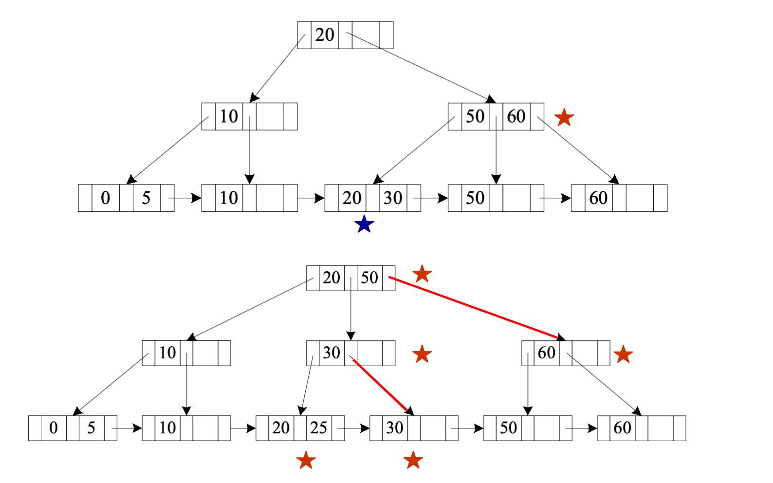
B+-Tree Example
手工插入例子
给出一组整数 B+-tree 插入过程,用来理解节点分裂和父节点更新。
初始 key 包括:
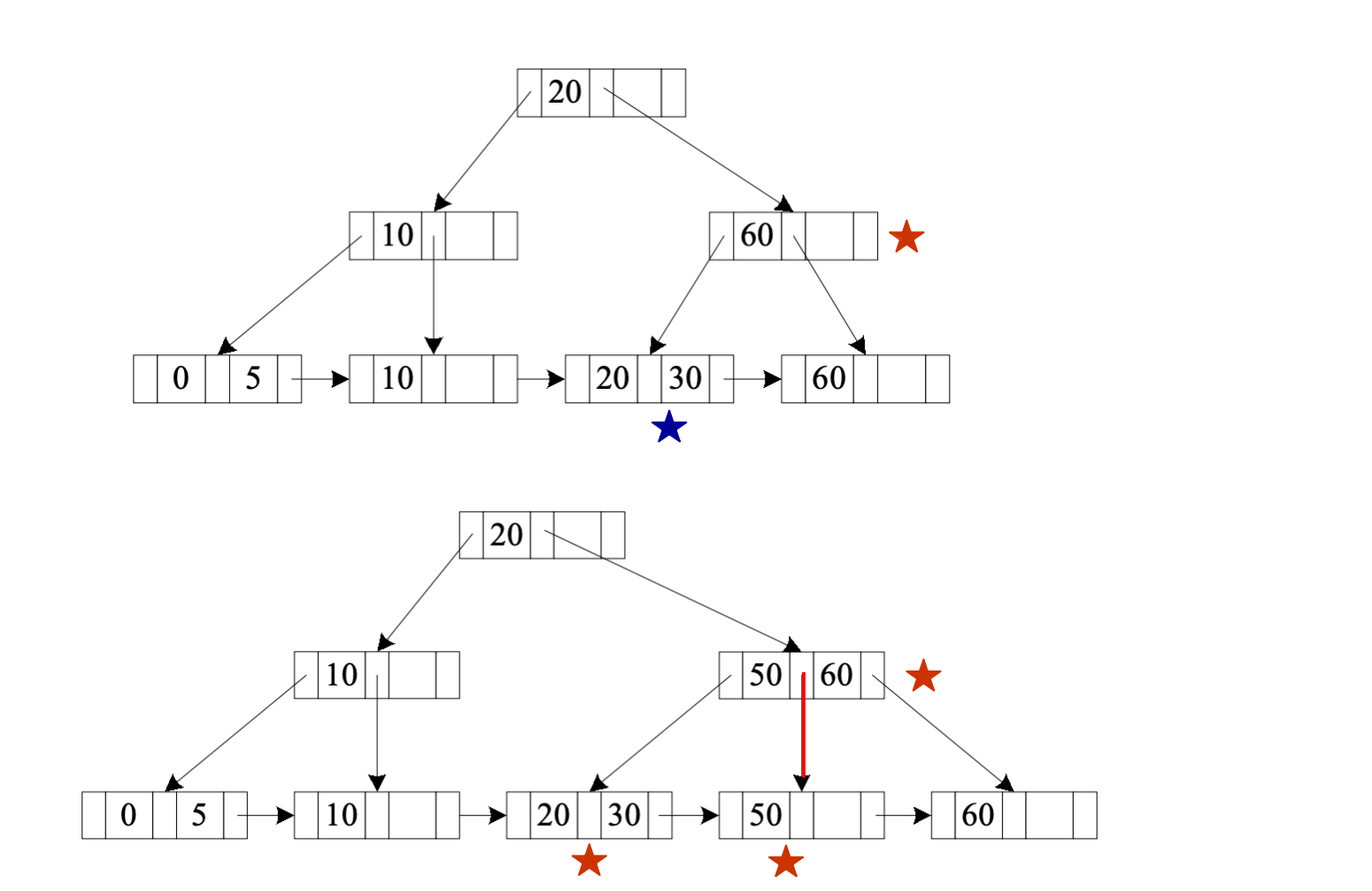
0, 5, 10, 20, 60插入 30
插入 30 后,对应 leaf 溢出,需要分裂。
变化重点:
- leaf 从原来的包含
20, 60,变成两个 leaf:20, 30和60 - 父节点需要插入新的分隔 key
- 如果父节点溢出,则继续 split
插入 50
插入 50 后:
50位于30和60之间- leaf split 后产生新的分隔 key
50 - parent 中增加用于导航的 key
插入 25
插入 25 后:
25落在20和30所在区域- leaf 分裂后可能导致 internal node 分裂
- root 可能从一个 key 变成两个 key,例如
20, 50
删除 60
删除 60 后:
- 叶子结点出现 underfull
- 与相邻叶子合并
- 父结点删除对应分隔 key
删除 10
删除 10 后:
- 叶子结点 underfull
- 通过向兄弟借 key 做 redistribution
- 父结点分隔 key 需要更新
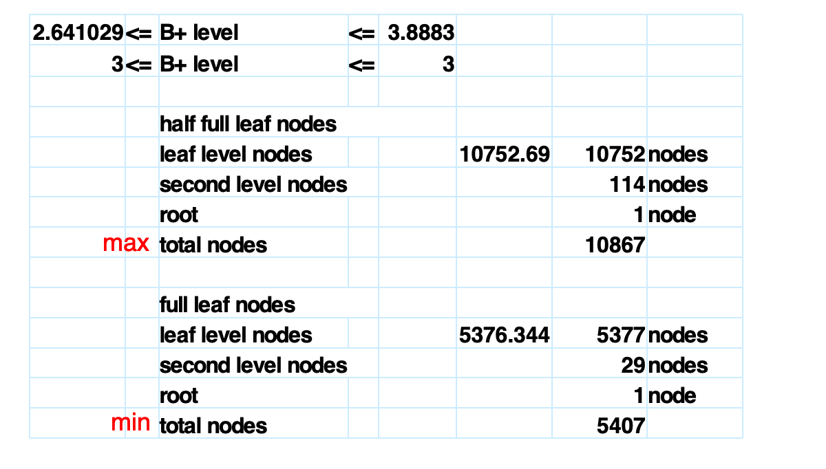
高度估算
person( pid char(18) primary key, name char(8), age smallint, address char(40));已知:
- block size = 4KB = 4096 bytes
- 共有 1,000,000 persons
- record size =
18 + 8 + 2 + 40 = 68 bytes
每个数据块可放记录数:
存储 100 万条记录需要数据块数:
B+-tree 索引中,假设:
- search key
pid大小为 18 bytes - pointer 大小为 4 bytes
- 一个节点保留 4 bytes 额外空间
fanout:
于是:
- internal node children 数:
94 ~ 187 - leaf values 数:
93 ~ 186
容量估算:
| 层数 | 最小容量 | 最大容量 |
|---|---|---|
| 2 levels | 2 × 93 = 186 | 187 × 186 = 34,782 |
| 3 levels | 2 × 94 × 93 = 17,484 | 187 × 187 × 186 = 6,504,234 |
| 4 levels | 2 × 94 × 94 × 93 = 1,643,496 | 187 × 187 × 187 × 186 = 1,216,291,758 |
所以 100 万条记录的 B+-tree index 高度在 3 到 4 层范围内。
如果按课件中的节点数估算,最终可以得到约 3 层索引结构。
NOTE这里的层数统计通常把 leaf level 也算进去。
做题时要看题目中的 height / level 定义是否包含 root 和 leaf。
B+-Tree File Organization
与 B+-Tree Index 的区别
B+-Tree Index 的 leaf node 保存:
(search-key, pointer-to-record)B+-Tree File Organization 的 leaf node 直接保存:
完整数据记录也就是说:
B+-tree file organization 用 B+-tree 本身组织数据文件,而不是只维护一个指向数据文件的索引。
好处:
- 插入、删除、更新后仍能保持数据记录的 clustering
- 支持按 search key 顺序访问数据
- 不需要额外从 leaf pointer 再跳到数据文件
代价:
- leaf node 中记录比 pointer 大得多
- 每个 leaf node 能容纳的记录数更少
- leaf 层节点数量更多
空间利用率
Leaf nodes 仍要求至少 half full。
但因为 leaf node 直接存 records,空间利用率更重要。
为提高空间利用率,可以在 split / merge 时涉及更多 sibling nodes。
例如:
在 redistribution 中涉及 2 个 sibling,可以在尽量避免 split / merge 的同时,让每个节点至少有约
floor(2n/3)个 entries。
这比单纯 half-full 更节省空间。
文件组织估算
继续使用 person 表:
person( pid char(18) primary key, name char(8), age smallint, address char(40));已知:
- record size = 68 bytes
- block size = 4096 bytes
每个 leaf node 最多可放:
个 records。
half-full 时,每个 leaf 至少约:
个 records。
存储 100 万条记录需要 leaf nodes:
- 最少:
- 最多:
non-leaf node fanout 仍是:
容量估算:
| 层数 | 最小容量 | 最大容量 |
|---|---|---|
| 2 levels | 2 × 30 = 60 | 187 × 60 = 11,220 |
| 3 levels | 2 × 94 × 30 = 5,640 | 187 × 187 × 60 = 2,098,140 |
| 4 levels | 2 × 94 × 94 × 30 = 530,160 | 187 × 187 × 187 × 60 = 392,352,180 |
| 5 levels | 2 × 94 × 94 × 94 × 30 = 49,835,040 | 187^4 × 60 ≈ 7.34e10 |
因此 100 万 records 在 B+-tree file organization 中通常 3 到 4 层即可覆盖。
B-Tree Index Files
B-Tree 与 B+-Tree 的区别
B-tree 和 B+-tree 类似,但有一个关键区别:
B-tree 中 search-key value 只出现一次。B+ tree 中 search-key value 可能出现在 non-leaf node 和 leaf node 中,同时中间节点的索引值不一定会出现在叶子结点上,他只要能起到区分两路,不一定会作为叶子结点的值出现,就比如删除以后可能就不在了。
也就是说:
- 如果某个 key 已经出现在 non-leaf node 中,它不会再出现在 leaf node 中
- non-leaf node 除了导航 pointer,还要保存指向实际记录或 bucket 的 pointer
因此 B-tree 可以减少 search key 的冗余存储。
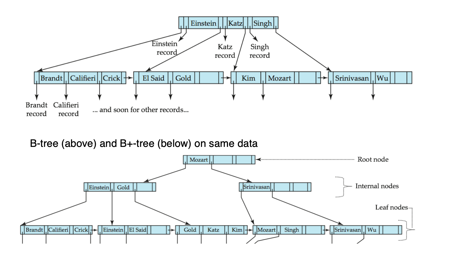
B-Tree 的优缺点
优点:
- 相比对应的 B+-tree,可能使用更少节点
- 有时在到达 leaf node 前就能找到目标 key
缺点:
- 只有少数 search-key values 能提前在 non-leaf node 找到
- non-leaf node 更大,因为还要存记录指针
- fanout 变小,树可能更深
- 插入和删除更复杂
- 实现难度比 B+-tree 高
结论:
实际数据库系统中,B-tree 的优势通常抵不过缺点,因此 B+-tree 更常用。
Secondary Index 的记录移动问题
在 B+-Tree File Organization 中,leaf node 直接保存完整 records。
因此,当 leaf node 发生 split / merge / redistribution 时,某些 records 的物理位置可能改变。
这会影响 secondary index 的设计。
直接保存 record pointer 的问题
假设有表:
person( pid char(18) primary key, name char(8), age smallint, address char(40));数据文件按 pid 组织成 B+-Tree File Organization。
也就是说:
-
primary index 的 search key 是
pid -
leaf node 中直接保存完整的
personrecords
同时,系统还建立了两个 secondary indices:
secondary index on agesecondary index on name如果 secondary index entry 直接保存 record pointer,那么可能长这样:
age index:20 -> block 100, slot 3
name index:Tom -> block 100, slot 3其中:
block 100, slot 3表示记录当前的物理位置。
假设这条记录是:
(pid = 005, name = Tom, age = 20, address = Hangzhou)此时,两个 secondary indices 都直接指向这条记录的物理地址。
现在向 B+-tree file 中插入新记录,导致某个 leaf node 分裂。
分裂前:
Leaf A:[001, 003, 005, 007]插入 pid = 004 后:
Leaf A:[001, 003, 004, 005, 007]节点放不下,需要 split:
Leaf A:[001, 003]
Leaf B:[004, 005, 007]于是 pid = 005 这条记录可能从:
block 100, slot 3移动到:
block 220, slot 2这时原来的 secondary index entry 就失效了:
age index:20 -> block 100, slot 3 // stale pointer
name index:Tom -> block 100, slot 3 // stale pointer为了保证正确性,所有指向这条记录的 secondary indices 都要更新:
age index:20 -> block 220, slot 2
name index:Tom -> block 220, slot 2如果表上有很多 secondary indices,记录每移动一次,就可能触发大量索引更新。
所以在 B+-tree file organization 中,node split 会变得很昂贵。课件把这个问题概括为:如果记录移动,所有存储 record pointer 的 secondary indices 都必须更新;解决办法是在 secondary index 中保存 primary-index search key,而不是 record pointer。
使用 primary-index search key 的方案
更稳定的做法是:
Secondary index entry 不保存物理 record pointer,而保存 primary-index search key。
在这个例子中,primary-index search key 是 pid。
因此 secondary index 可以写成:
age index:20 -> 005
name index:Tom -> 005查询 age = 20 时,流程变成两步:
1. 通过 age index 找到 pid: age = 20 -> pid = 005
2. 再通过 primary index 找到真实记录: pid = 005 -> current record location也就是说:
secondary index -> primary key -> primary index -> record现在即使 pid = 005 的记录因为 leaf split 从:
block 100, slot 3移动到:
block 220, slot 2Secondary index 仍然不需要修改:
age index:20 -> 005
name index:Tom -> 005因为 pid = 005 没有变。
只需要 primary index 能找到这条记录的新位置即可。
代价与收益
这种设计的本质是一个 trade-off。
| 方案 | Secondary index 保存内容 | 查询代价 | 记录移动代价 |
|---|---|---|---|
| 直接保存 record pointer | 物理地址,如 block 100, slot 3 | 低 | 高,所有相关 secondary indices 都要更新 |
| 保存 primary-index search key | 主键,如 pid = 005 | 较高,需要再查 primary index | 低,记录移动时 secondary index 不变 |
所以:
保存 record pointer 查询更直接,但对记录移动很敏感;保存 primary-index search key 查询多走一步,但对记录移动更稳定。
如果 primary-index search key 本身不唯一,还需要额外加上 record-id 来唯一定位记录。
例如,如果 primary index 建在 dept_name 上:
dept_name = CS可能对应很多 records。
这时 secondary index 不能只保存:
age = 20 -> CS因为无法唯一确定是哪一条记录。
需要保存类似:
age = 20 -> (CS, record-id)其中 record-id 用来区分同一个 primary search key 下的不同记录。
Variable Length Keys 与 Prefix Compression
Variable Length Strings as Keys
如果 search key 是变长字符串,会带来两个问题:
- 每个节点能容纳的 entry 数不固定
- fanout 变成 variable fanout
此时 split 的判断标准不应只看 pointer 数量,而应看:
节点空间利用率。
也就是节点是否超过页大小,或者是否低于最低空间占用要求。
Prefix Compression
对字符串索引,可以使用 prefix compression(前缀压缩)。
Internal node 中不一定要保存完整 key,只要保存足够区分相邻子树的前缀即可。
例如:
SilasSilberschatz可以用:
Silb来区分对应子树。
Leaf node 中也可以压缩共同前缀,减少空间。
TIPprefix compression 的核心是:
internal node 的 key 只用于导航,不一定需要等于完整 search key。
只要能正确区分左右子树,就足够。
Indices on Multiple Keys
多个单属性索引
考虑查询:
select IDfrom instructorwhere dept_name = 'Finance' and salary = 80000;如果只有单属性索引,可以有三种策略。
策略一:使用 dept_name 索引
- 找到所有
dept_name = 'Finance'的记录 - 再在内存中测试
salary = 80000
策略二:使用 salary 索引
- 找到所有
salary = 80000的记录 - 再在内存中测试
dept_name = 'Finance'
策略三:两个索引都用
- 用
dept_name索引得到一组 record pointers - 用
salary索引得到另一组 record pointers - 对两组 pointers 求交集
- 再访问交集对应记录
策略三要求索引能返回 record pointers。
Composite Search Key
Composite search key(复合搜索键) 椏。前2. 由多个属性组成。
例如:
(dept_name, salary)复合键按字典序比较。
对于 (a1, a2) 和 (b1, b2):
当且仅当:
a1 < b1,或a1 = b1且a2 < b2
复合索引能高效支持什么查询
假设有索引:
(dept_name, salary)它可以高效处理:
where dept_name = 'Finance' and salary = 80000因为两个属性都按照复合键顺序定位。
也可以高效处理:
where dept_name = 'Finance' and salary < 80000因为先固定第一维 dept_name,再在第二维 salary 上做范围扫描。
但它不能高效处理:
where dept_name < 'Finance' and salary = 80000原因是:
- 字典序首先按
dept_name排序 dept_name < 'Finance'会覆盖许多不同部门- 在这些部门内部才按
salary排序 - 所以会取出大量满足第一条件但不满足第二条件的记录
WARNING复合索引的顺序非常重要。
(dept_name, salary)和(salary, dept_name)支持的高效查询模式不一样。
非唯一搜索键的处理
如果某个 search key ai 不唯一,可以建立唯一复合索引:
(ai, Ap)其中 Ap 可以是:
- primary key
- record ID
- 其他能保证唯一性的属性
查找:
ai = v可以转化为复合键上的范围查询:
(v, -∞) 到 (v, +∞)优点:
- 插入删除实现更简单
- 每个 index entry 唯一
- widely used
代价:
- key 更长,有额外存储开销
- 获取实际记录可能需要更多 I/O
- clustering index:访问大多是顺序的
- non-clustering index:每条记录可能一次随机 I/O
Indexing in Main Memory
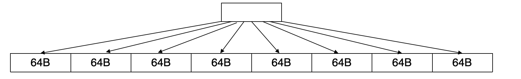
主存中的随机访问比磁盘和 Flash 便宜很多,但仍然比 cache read 贵。
问题在于:
在一个很大的 B+-tree node 中二分查找 key,可能造成多次 cache miss。
因此主存索引需要 cache-conscious data structure。
一种思路是:
- 对磁盘访问:使用大节点,减少磁盘 I/O
- 对 cache 访问:在节点内部用适合 cache line 的小结构组织数据
例如:
- 磁盘页大小可能是 4KB
- cache line 可能是 64B
- 如果节点内部只是大数组,二分查找可能跳到多个 cache line
- 可以把节点内部组织成小树或分块结构,让访问更符合 cache locality
Bulk Loading and Bottom-Up Build
逐条插入的问题
如果一次要加载大量 index entries,逐条插入 B+-tree 代价很高。
原因:
- 每条插入至少访问一个 leaf
- 如果 leaf level 不能放入内存,几乎每条插入都可能带来 I/O
- 对大量数据做 bulk loading 时效率很差
Sorted Insertion
第一种优化方式:
- 先把 entries 排序
- 再按排序顺序插入 B+-tree
好处:
- 连续插入通常落在同一 leaf 或相邻 leaf
- I/O 性能明显改善
问题:
- 许多 leaf nodes 最后只有 half full
- 空间利用率不一定好
Bottom-Up B+-Tree Construction
第二种优化方式是 bottom-up build。
步骤:
- 先排序所有 index entries
- 从 leaf level 开始顺序创建 B+-tree
- 再逐层向上构建 internal levels
- 整棵树按顺序 I/O 写入磁盘
这是大多数数据库 bulk-load 工具采用的方式。
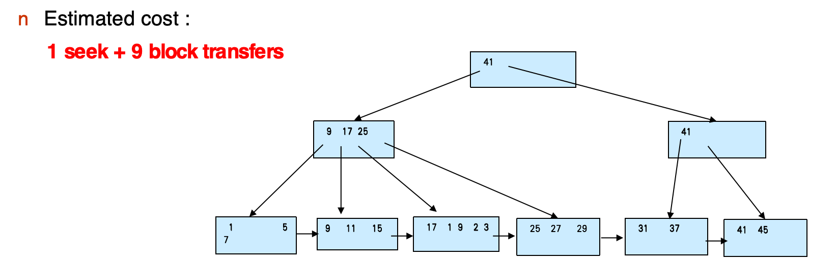
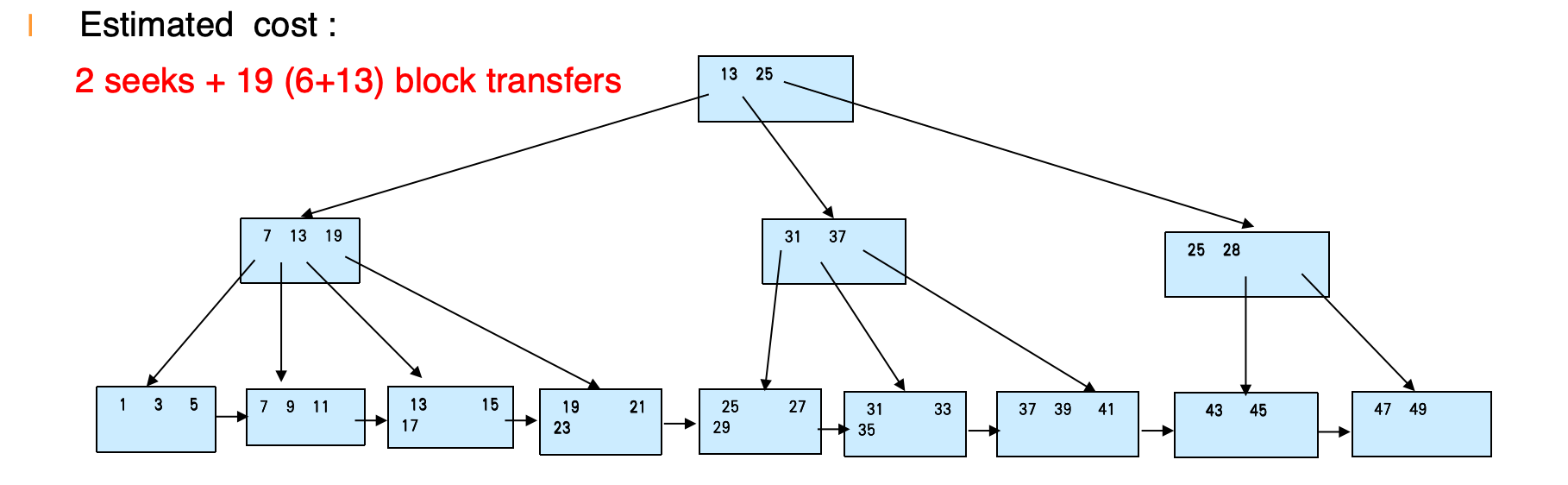
例子:fanout n = 4,为 16 个 entries 建树。
原始 entries:
23 25 27 29 1 5 7 9 11 31 37 41 45 15 17 19排序后:
1 5 7 9 11 15 17 19 23 25 27 29 31 37 41 45再从 leaf level 开始逐层构造 B+-tree。
估算代价:
1 seek + 9 block transfers说明: 时叶子最多 个 entry,叶层块数为 。上一层 internal 节点每个最多 4 个指针,需要 块,root 为 1 块。顺序写入共 次 block transfer,顺序写只需 1 次 seek。
Bulk Insert
如果已有一棵 B+-tree,又要批量插入一批 entries,可以:
- 对新 entries 排序
- 把原树和新 entries 合并
- 使用 bottom-up build 重新构造一棵新 B+-tree
例子:向前一棵 B+-tree 插入 9 个 entries:
21 33 35 39 43 47 49 3 13排序后:
3 13 21 33 35 39 43 47 49估算代价:
2 seeks + 19 block transfers说明:合并后共有 个 entry。顺序扫描旧树的 leaf level 需要读取 个 leaf 块;重建新树时叶层为 块,internal 层为 块,root 为 1 块,共写入 块。总 block transfer 为 ,顺序读旧树与顺序写新树各 1 次 seek。
这也是 LSM-tree 中合并多个 B+-tree 的思想基础。
Indexing on Flash
Flash 上的索引设计和磁盘不同。
Flash 的特点:
- Random I/O 比磁盘低很多,读写通常为几十微秒级
- 不能原地覆盖写入
- 写入最终需要 erase,而 erase 代价更高
- 最优 page size 通常比磁盘小
因此:
- B+-tree 上的随机读不像磁盘上那么致命
- 但频繁 page overwrite 会造成写放大和 erase 成本
- bulk-loading 仍然有用,因为它减少 page erase
- LSM-tree 等 write-optimized tree 被用于减少 Flash 上的 page writes
TIPFlash 上的核心问题从“避免随机寻道”转向“减少写入和擦除”。
Write Optimized Indices
为什么普通 B+-Tree 写入不友好
B+-tree 对读很友好,但对写密集 workload 可能表现很差。
假设 internal nodes 都在内存中,插入仍然通常需要:
- 找到 leaf
- 修改 leaf page
- 写回 leaf page
也就是:
每次插入大约一次 leaf I/O。
在磁盘上,这意味着每块磁盘每秒插入数可能低于 100。
在 Flash 上,这意味着每次插入都可能造成 page overwrite。
两类降低写成本的方法:
- Log-Structured Merge Tree(LSM-tree)
- Buffer Tree
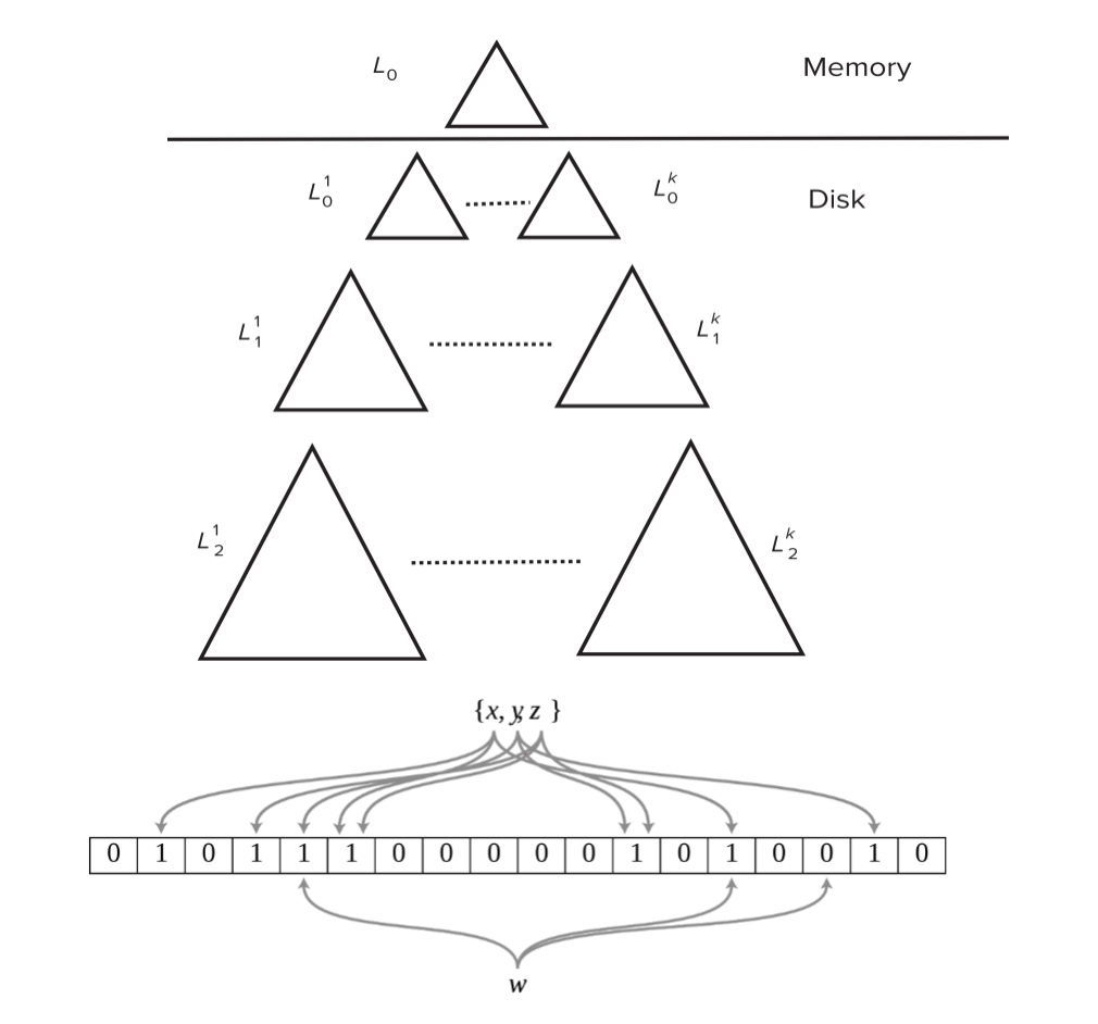
Log-Structured Merge Tree
LSM-tree 先只考虑 insert 和 query。
基本结构:
L0 tree:内存中的树L1 tree:磁盘中的树L2 tree:更大的磁盘树- 更多层以此类推
插入过程:
- 新记录先插入内存中的
L0 tree - 当
L0 tree满时,将其和磁盘上的L1 tree合并 - 合并时用 bottom-up build 构造新的
L1 tree - 当
L1 tree超过阈值,再合并进L2 tree Li+1的大小阈值通常是Li的k倍
LSM 的优势:
- 插入主要转化为顺序 I/O
- leaf nodes 通常是满的,空间浪费少
- 相比普通 B+-tree,单条记录写入 I/O 更少
LSM 的缺点:
- 查询需要搜索多个 tree
- 每层合并时会多次复制已有内容
- 读放大和写放大之间存在权衡
Stepped-Merge Index
Stepped-merge index 是 LSM-tree 的一种变体。
它在每个磁盘层保存 k 棵树。
规则:
- 当某一层已有
k个 indices 时 - 将它们合并成下一层的一个 index
优点:
- 比普通 LSM-tree 写成本更低
缺点:
- 查询更贵,因为每层可能有多棵树要查
优化方式:
- 为每棵树计算 Bloom filter
- Bloom filter 放在内存中
- 点查询时,只有 Bloom filter 返回 positive 的树才真正访问
LSM 中的删除与更新
LSM 中删除不直接原地删除记录,而是加入特殊的 delete entry。
也叫:
- tombstone
- delete marker
查询时:
- 可能同时找到原记录和 delete entry
- 系统必须只返回没有被 delete entry 匹配删除的记录
合并时:
- 如果 delete entry 与原记录匹配
- 二者都可以被丢弃
更新可以看成:
delete old record + insert new recordLSM 最初用于磁盘索引,也适合 Flash,因为它能减少 erase。
stepped-merge 变体被许多 BigData 存储系统使用,例如 BigTable、Cassandra、MongoDB,也出现在 LevelDB 和 MyRocks 等系统中。
Buffer Tree
Buffer tree 的核心思想是:
在 B+-tree 的 internal node 中加入 buffer,用来暂存 inserts。
过程:
- 插入先进入上层节点的 buffer
- 当 buffer 满时,批量向下层移动
- 每次向下移动许多 records
- 单条记录分摊的 I/O 成本下降
优点:
- 查询额外开销比 LSM 小
- 可以和多种 tree index structure 结合
- PostgreSQL 的 GiST indices 中使用了类似思想
缺点:
- 比 LSM-tree 产生更多 random I/O
NOTELSM-tree 更像把随机写转成顺序批量合并。
Buffer tree 更像在树节点中加缓冲,把小写入攒成批量下推。
Bitmap Indices
适用场景
Bitmap index 是一种适合多属性查询的特殊索引。
它通常用于取值种类较少的属性,例如:
- gender
- country
- state
- income-level
要求:
- relation 中的 records 可以从 0 开始顺序编号
- 给定编号
n后,能快速取出第n条记录 - 如果记录是 fixed-size,这件事尤其容易
Bitmap index 不太适合高基数属性,例如:
- 学号
- 身份证号
- UUID
因为每个不同值都要一个 bitmap,空间会爆炸。
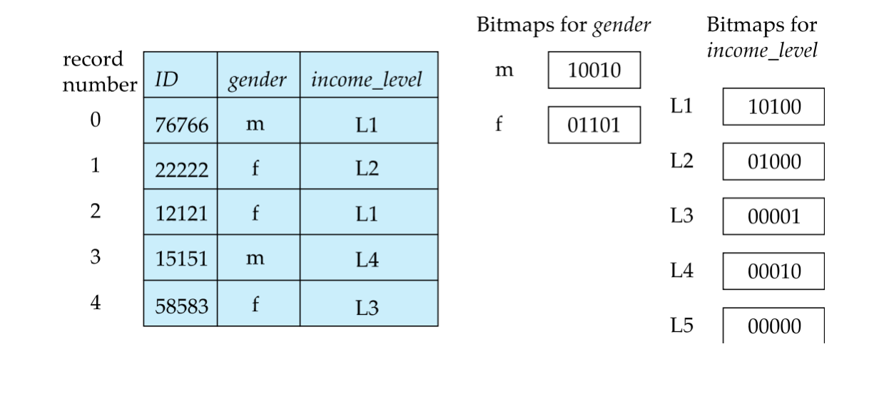
基本结构
最简单的 bitmap index:
对某个属性的每个取值建立一个 bitmap。
如果 relation 有 N 条记录,每个 bitmap 就有 N 个 bits。
对某个值 v 的 bitmap:
- 第
i位为 1:第i条记录在该属性上的值是v - 第
i位为 0:第i条记录在该属性上的值不是v
位运算查询
Bitmap index 特别适合多个属性上的组合查询。
查询可以转化为位运算:
- intersection:AND
- union:OR
- negation:NOT
例如:
100110 AND 110011 = 100010100110 OR 110011 = 110111NOT 100110 = 011001如果要查:
Males with income level L1可以做:
gender = male 的 bitmapANDincome_level = L1 的 bitmap例子:
10010 AND 10100 = 10000结果 bitmap 中为 1 的位置,就是满足条件的记录编号。
TIP如果只需要 count,不需要取出完整 tuple,bitmap index 更快。
因为 count 只需要统计结果 bitmap 中 1 的个数。
空间与计算优势
Bitmap 通常很小。
如果每条 record 是 100 bytes:
- 一个 bitmap 对每条 record 只需要 1 bit
- 一个 bitmap 的空间约为 relation 空间的
1/800
如果属性有 8 个不同取值:
- 8 个 bitmaps 总空间约为 relation 的 1%
Bitmap 的计算也很快:
- bitmaps 会打包进机器字
- 一个 32-bit 或 64-bit CPU 指令可以同时处理 32 或 64 位
- 100 万 bit 的 bitmap,只需约 31,250 次 32-bit AND 指令
统计 1 的个数可以用预计算表:
- 为 0 到 255 的每个 byte 预存其二进制表示中 1 的个数
- 扫描 bitmap 的每个 byte
- 查表并累加
也可以用两个 byte 做表,速度更快,但内存开销更大。