Nonlinear Systems and Phenomena - Be Happy Every Day

Overview#

Chapter 7 研究 solution curves 的定性行为。核心问题有四个：

Equilibrium / Critical points：系统在哪些点不动；
Stability：从这些点附近出发，轨道会靠近、远离，还是绕着转；
Linearization：复杂 nonlinear system 在 critical point 附近，常常可以先看 Jacobian 对应的 linear system；
Ecological interpretation：predator-prey / competition / cooperation 等模型里，critical points 与 phase portrait 直接决定长期种群命运。

\boxed{\text{find critical points } \to \text{ draw phase line/phase portrait } \to \text{ classify stability}}

Contents#

Overview
Contents
Equilibrium Solutions and Stability
Stability and the Phase Plane
Linear and Almost Linear Systems
Ecological Models: Predators and Competitors
Example
- A more complicated scenario

Equilibrium Solutions and Stability#

Autonomous first-order equations#

最简单的非线性情形是

\frac{dx}{dt}=f(x).

这叫做 autonomous first-order differential equation，因为右端不显含 $t$ 。

这类方程的优势是：
只看 $f(x)$ 的符号，就能读出解的方向与长期行为。

Critical points and equilibrium solutions#

若

f(c)=0,

则常值函数

x(t)\equiv c

满足方程，因此：

$c$ 叫做 critical point；
$x(t)\equiv c$ 叫做 equilibrium solution。

所以一维自治方程的第一步永远是：

\boxed{f(x)=0}

先把所有 critical points 找出来。

Stability in Lyapunov’s sense#

设 $x=c$ 是一个 critical point。

$x=c$ stable，如果对任意 $\varepsilon>0$ ，都存在 $\delta>0$ ，使得
$|x_0-c|<\delta$
蕴含
$|x(t)-c|<\varepsilon,\qquad \forall t>0.$
若不满足这个条件，则称为 unstable。

几何上：

从 equilibrium 附近出发的轨道，若一直 stay nearby，则这个 equilibrium 是 stable 的。

若更进一步有

x(t)\to c\qquad (t\to+\infty),

则它叫做 asymptotically stable。

One-dimensional phase line#

对

\frac{dx}{dt}=f(x),

做 phase line 的步骤非常固定：

解 $f(x)=0$ ；
在各区间判断 $f(x)$ 的正负；
用箭头表示解的运动方向：

$f(x)>0$ ：箭头向右；
$f(x)<0$ ：箭头向左。

因此：

两侧箭头都指向 critical point $\Rightarrow$ stable，通常还是 asymptotically stable；
两侧箭头都远离 critical point $\Rightarrow$ unstable；
一侧靠近、一侧远离 $\Rightarrow$ semistable。

Logistic equation#

考虑 logistic equation

\frac{dx}{dt}=kx(M-x),\qquad k>0,\ M>0.

Critical points#

令右端为 0：

kx(M-x)=0

得到

x=0,\qquad x=M.

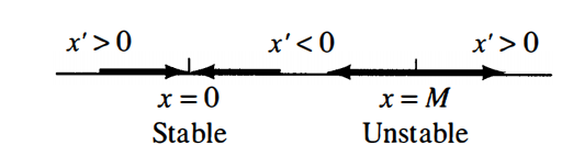
Phase line and stability#

设

f(x)=kx(M-x).

分区间判号：

$x<0$ 时， $f(x)<0$ ；
$0<x<M$ 时， $f(x)>0$ ；
$x>M$ 时， $f(x)<0$ 。

$x=0$ 是 unstable；
$x=M$ 是 stable，实际上还是 asymptotically stable。

Explicit solution and long-time behavior#

若 $x(0)=x_0$ ，则

x(t)=\frac{Mx_0}{x_0+(M-x_0)e^{-kMt}}.

因此：

若 $x_0>0$ ，则 $x(t)\to M;$
若 $x_0=0$ 或 $x_0=M$ ，则停在对应 equilibrium；
若 $x_0<0$ ，则分母会在有限时间变为 0，解发散到 $-\infty$ 。

Explosion/Extinction Equation#

现在把 logistic 中的符号反过来，考虑

\frac{dx}{dt}=kx(x-M),\qquad k>0,\ M>0.

它仍有两个 critical points：

x=0,\qquad x=M.

但 phase line 完全不同。设

f(x)=kx(x-M).

分区间判号：

$x<0$ 时， $x<0$ 且 $x-M<0$ ，故 $f(x)>0$ ；
$0<x<M$ 时， $f(x)<0$ ；
$x>M$ 时， $f(x)>0$ 。

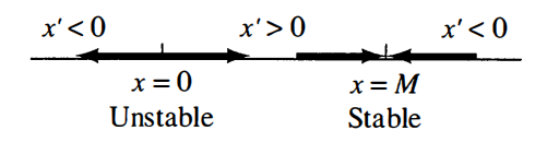
所以 phase line 为

于是：

$x=0$ 是 stable；
$x=M$ 是 unstable。

若用显式解

x(t)=\frac{Mx_0}{x_0+(M-x_0)e^{kMt}},

可进一步得到：

若 $x_0<M$ ，则 $x(t)\to 0$ ；
若 $x_0=M$ ，则恒等于 $M$ ；
若 $x_0>M$ ，则在有限时间 blow up 到 $+\infty$ 。

同样是两个 critical points，稳定性可能因为一个符号变化而完全翻转。

Logistic population with harvesting#

带 harvesting 的 logistic 模型写成

\frac{dx}{dt}=ax-bx^2-h,

a 也可写成

\frac{dx}{dt}=kx(M-x)-h.

其中：

$kx(M-x)$ 是自然增长；
$h$ 是每单位时间固定 harvest 的个体数。

Critical points and threshold#

令右端为零：

-kx^2+kMx-h=0.

当

4h<kM^2

时，有两个实根：

H,N=\frac{kM\pm\sqrt{(kM)^2-4kh}}{2k} =\frac12\left(M\pm\sqrt{M^2-\frac{4h}{k}}\right),

并且

0<H<N<M.

此时方程可因式分解为

\frac{dx}{dt}=k(N-x)(x-H).

于是 phase line 是

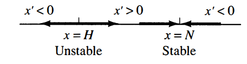
因此：

$x=H$ 是 unstable；
$x=N$ 是 stable。

这里 $x(t)\equiv H$ 很重要，它叫做 threshold solution：

若 $x_0>H$ ，则解最终趋于 $N$ ；
若 $x_0<H$ ，则种群会被捕捞拖向灭绝。

所以 $H$ 不是长期极限，而是“分界线”。

Three parameter regimes#

Case 1: $4h<kM^2$

有两个不同实根 $H<N$ 。

$H$ unstable；
$N$ stable；
若 $x_0>H$ ，则 $x(t)\to N$ ；
若 $x_0<H$ ，则种群灭绝。

Case 2: $4h=kM^2$

两个根合并成一个：

H=N=\frac M2.

这时

\frac{dx}{dt}=-k\left(x-\frac M2\right)^2.

phase line 为

\leftarrow\quad \frac M2\quad \leftarrow

因此 $x=\frac M2$ 是 semistable：

从右边看，解靠近它；
从左边看，解远离它。

Case 3: $4h>kM^2$

没有实根，因此没有 equilibrium solutions。

这时自然增长项的最大值也不足以抵消 harvesting，系统对所有初值都会走向灭绝。

Concrete example#

若取

k=1,\qquad M=4,\qquad h=3,

则模型为

\frac{dx}{dt}=x(4-x)-3.

二次方程

-x^2+4x-3=(3-x)(x-1)=0

给出

H=1,\qquad N=3.

若 $x$ 的单位是 “hundreds of fish”，则：

threshold population = 100 fish；
new limiting population = 300 fish。

所以：

初始鱼群多于 100 条，长期趋于 300 条；
初始鱼群少于 100 条，会被完全捕捞掉。

Bifurcation and Dependence on Parameters#

当我们把 $h$ 当成连续变化的参数时，critical points 的数目会发生突变：

$h<4$ ：有两个 critical points；
$h=4$ ：只有一个 semistable critical point；
$h>4$ ：没有 critical points。

这种参数连续变化，而系统的 qualitative behaviour 突然改变的现象，叫做 bifurcation。

在方程

\frac{dx}{dt}=x(4-x)-h

中，critical points 满足

c=2\pm\sqrt{4-h}.

等价地可写成

(c-2)^2=4-h.

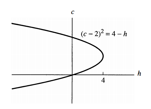
这是一条抛物线，给出了所有“参数 $h$ 与对应 equilibrium $c$ ”的关系，这张图就叫 bifurcation diagram。

critical points 的位置、数目与稳定性都可能依赖于参数；当参数穿过某个临界值时，系统结构会突然改变。

Stability and the Phase Plane#

From one-dimensional phase line to phase plane#

二维自治系统写成

\dot x=F(x,y),\qquad \dot y=G(x,y).

这时未知量不再活在一条数轴上，而是活在 xy phase plane 里。

与 1D phase line 相比，2D phase plane 的轨道行为更复杂。轨道可以：

靠近 critical point；
远离 critical point；
围着 critical point 转圈；
螺旋地靠近或远离；
甚至趋向某个 closed orbit / limit cycle。

通过 phase portrait 来判断 trajectories 在 critical points 附近如何运动。

Critical points in the plane#

若

F(x^*,y^*)=0,\qquad G(x^*,y^*)=0,

则 $(x^*,y^*)$ 是系统的 critical point / equilibrium point。

求 critical points 的办法仍然非常朴素：

\boxed{F(x,y)=0,\qquad G(x,y)=0}

解这个代数系统。

Stable vs. asymptotically stable#

对二维系统，Lyapunov stability 的定义和一维本质相同，只是现在的距离要用二维向量来理解。

几何上：

stable：从 nearby point 出发的轨道始终 stay close；
asymptotically stable：不仅 stay close，而且随着 $t\to\infty$ 真正靠近 critical point；
unstable：从 nearby point 出发会被甩开。

这里要特别注意：

在二维系统里，stable 不一定 asymptotically stable。

因为轨道可能只是绕着 critical point 转圈，不会跑远，但也不会收敛进去。
典型例子就是 center。

Typical local behaviors#

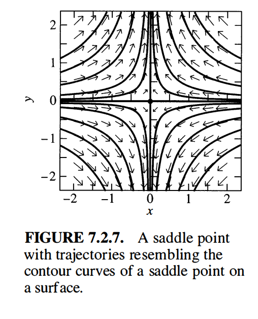
Saddle point#

某些方向靠近，某些方向远离；
一般是 unstable。

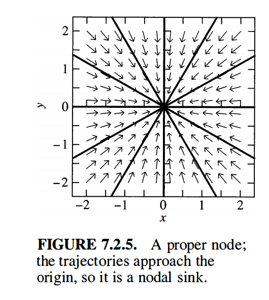
Node#

轨道大致沿若干方向一起流向或远离 critical point；
若都流入，则 stable / asymptotically stable；
若都流出，则 unstable。

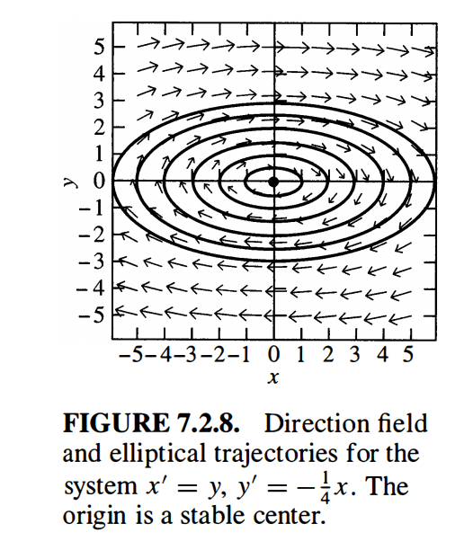
Center#

附近轨道是闭曲线，围着 critical point 打转；
stable but not asymptotically stable。

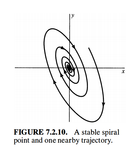
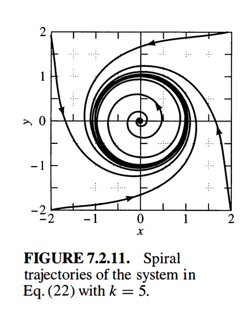
Spiral point#

轨道螺旋式进入或离开 critical point；
inward spiral 是 stable 且 asymptotically stable；
outward spiral 是 unstable。

Limit cycle#

轨道不趋向 critical point，而是趋向一个 closed trajectory；
这是二维 nonlinear system 里很有代表性的现象。

Examplee#

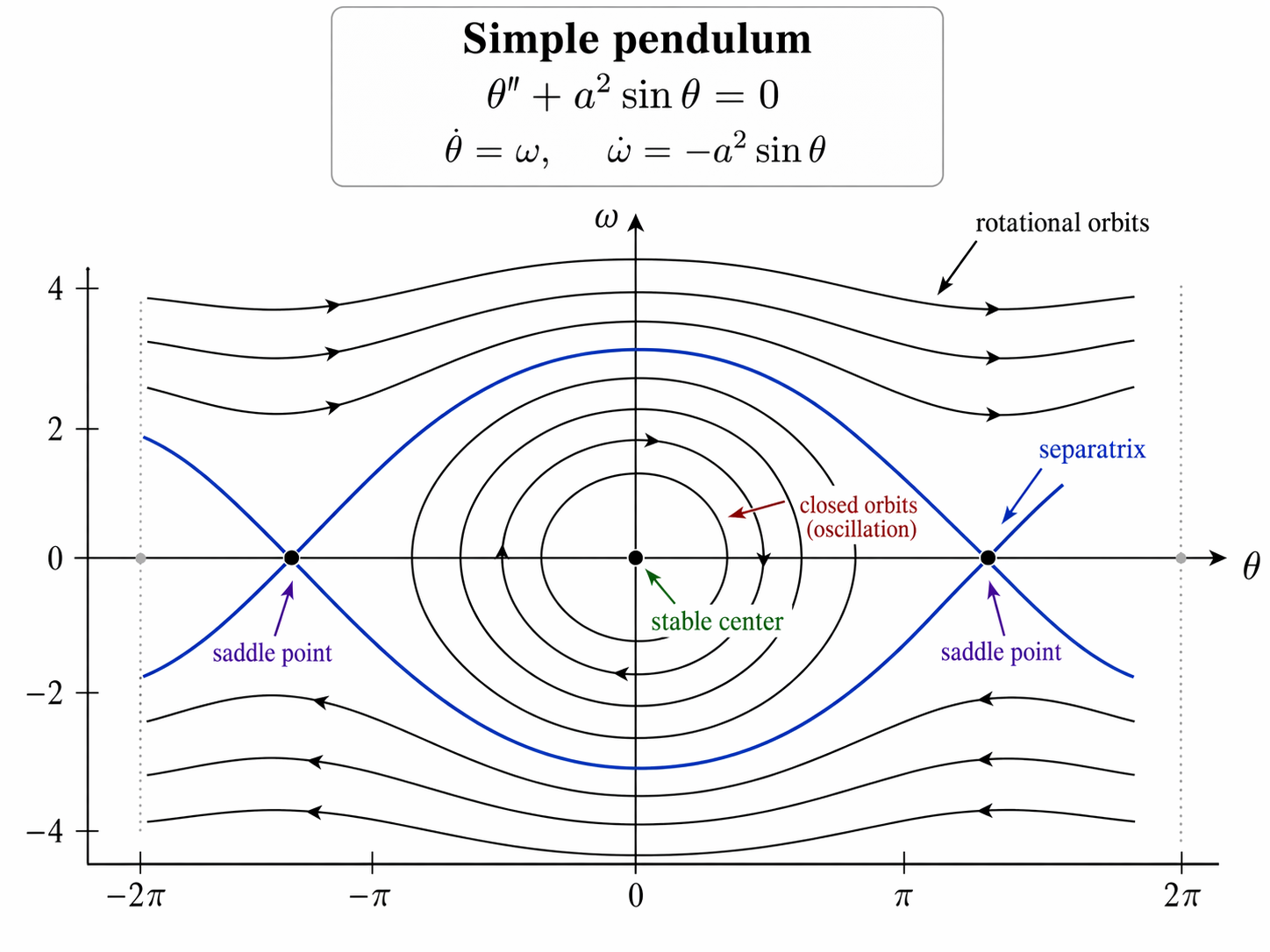
a simple frictionless pendulum

课上额外讲了 simple pendulum：

\theta''+a^2\sin\theta=0.

令

\omega=\theta',

则可改写为二维自治系统

\begin{cases} \dot\theta=\omega,\\ \dot\omega=-a^2\sin\theta. \end{cases}

这是一个典型的 2D phase-plane model。

物理解释

$\theta$ ：摆角；
$\omega$ ：角速度。

相图的三类典型轨道

小振幅闭轨道：对应来回摆动；
外侧开轨道：对应连续转圈；
经过 saddle 的 separatrix：分隔“摆动”和“转圈”两类行为。

因此 simple pendulum 是理解 phase portrait 的极好例子：
同一个系统里，closed orbit、saddle、separatrix 都会同时出现。

Linear and Almost Linear Systems#

Linear systems and linearization#

先看二维线性系统

\begin{cases} \dot x=ax+by,\\ \dot y=cx+dy. \end{cases}

也就是

\dot{\mathbf x}=A\mathbf x,\qquad A= \begin{pmatrix} a&b\\ c&d \end{pmatrix}.

对于一般 nonlinear system，如果 $\mathbf c$ 是一个 critical point，那么总可以先做平移

\mathbf u=\mathbf x-\mathbf c,

把 critical point 移到原点，再在原点附近用 Jacobian 做 linearization：

\dot{\mathbf u}=J(\mathbf c)\mathbf u+\text{higher-order terms}.

因此：

研究 nonlinear system 在 isolated critical point 附近的行为，第一步往往就是看 Jacobian 的 eigenvalues。

Three canonical cases#

二维线性系统在 Jordan canonical form 下归成三类：

Case I

\begin{pmatrix} \lambda&0\\ 0&\mu \end{pmatrix}

对应两个实特征值。轨道满足

y=Cx^{\mu/\lambda}

以及坐标轴方向上的特解。

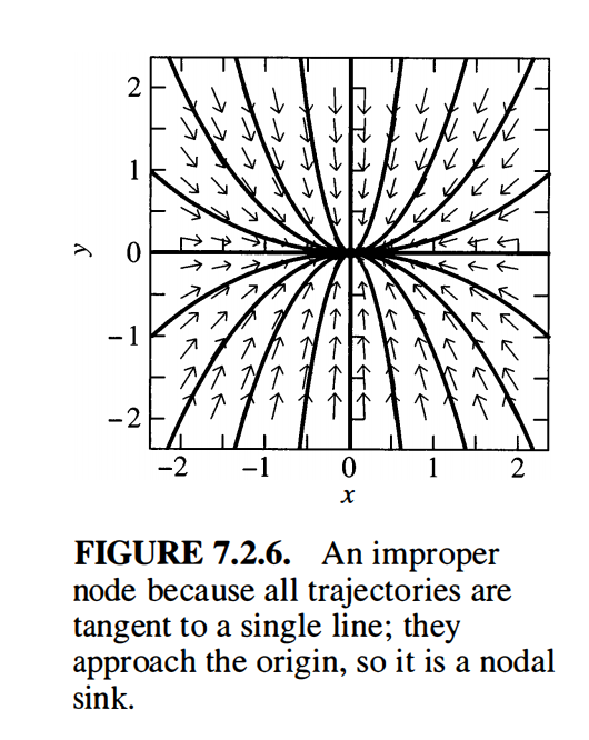
Case II

\begin{pmatrix} \lambda&1\\ 0&\lambda \end{pmatrix}

对应重特征值但只有一个 eigenvector 的 Jordan block。
典型轨道会表现为 improper node。

Case III

\begin{pmatrix} \alpha&-\beta\\ \beta&\alpha \end{pmatrix}, \qquad \beta\neq 0

对应共轭复特征值

\alpha\pm i\beta.

此时相图是 center 或 spiral。

Classification by eigenvalues#

对

A= \begin{pmatrix} a&b\\ c&d \end{pmatrix},

特征值为

\lambda_{1,2}=\frac{(a+d)\pm\sqrt{(a+d)^2-4(ad-bc)}}{2}.

因此 classification 完全取决于：

特征值是 real 还是 complex；
是否 equal；
real part 的 sign 是 positive 还是 negative。

常用分类总结#

两个实特征值，异号

\lambda_1\lambda_2<0

则是 saddle point，一定 unstable。

两个实特征值，同号

都负：stable node；
都正：unstable node。

distinct same-sign real eigenvalues 常表现为 improper node；
若 repeated eigenvalue 且有两条独立特征方向，则常表现为 proper node / star。

一对复共轭特征值

\lambda=\alpha\pm i\beta,\qquad \beta\neq 0

$\alpha<0$ ：stable spiral；
$\alpha>0$ ：unstable spiral；
$\alpha=0$ ：center（线性系统里 stable but not asymptotically stable）。

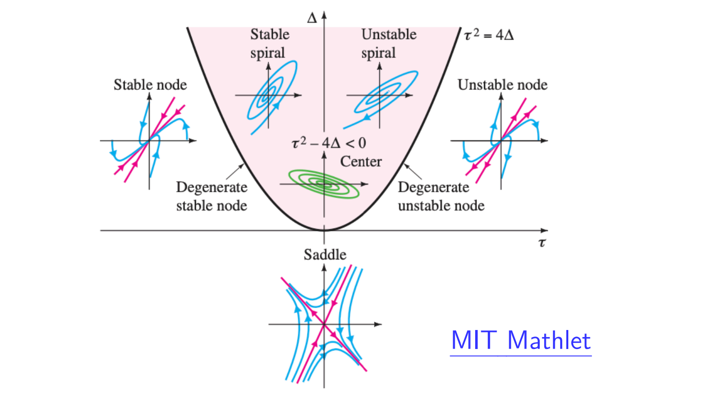
Trace-determinant diagram#

设

\tau=\operatorname{tr}(A)=a+d,\qquad \Delta=\det(A)=ad-bc.

则特征值满足

\lambda^2-\tau\lambda+\Delta=0.

这给出著名的 trace-determinant diagram：

$\Delta<0$ ：一定是 saddle；
$\Delta>0,\ \tau^2-4\Delta>0$ ：两个实根，node；
$\Delta>0,\ \tau^2-4\Delta<0$ ：一对复根，spiral 或 center；
$\tau=0,\ \Delta>0$ 且复根：center（线性情形）。

具体地：

$\tau<0$ ：实部偏负，趋于 stable；
$\tau>0$ ：实部偏正，趋于 unstable。

所以 trace-determinant plane 可以一张图把 node / saddle / center / spiral 全部总结出来。 trace-determinant diagram

Example#

$\dot x=2x+7y,\ \dot y=x-4y$

写成矩阵：

A= \begin{pmatrix} 2&7\\ 1&-4 \end{pmatrix}.

特征方程为

\lambda^2+2\lambda-15=0 =(\lambda-3)(\lambda+5).

所以特征值是

\lambda_1=3,\qquad \lambda_2=-5.

两特征值异号，因此原点是 saddle point，而且是 unstable。

这个例子很适合记住：

2D linear system 的 local behavior，本质上又回到了 matrix eigenvalue problem。

Almost linear systems#

一般 nonlinear system 在 isolated critical point 附近可以写成

\dot{\mathbf u}=A\mathbf u+\mathbf r(\mathbf u), \qquad \mathbf r(\mathbf u)=o(|\mathbf u|).

这种情形叫做 almost linear system。

思想上就是：

线性部分 $A\mathbf u$ 决定主要局部结构；
nonlinear remainder 只是在足够靠近 critical point 时做“小修正”。

因此，多数情况下，nonlinear system 与 linearization 具有相同的局部 type 和 stability。

Two tricky scenarios#

线性化并不是在所有情况下都完全决定局部行为。真正麻烦的是两类：

equal real eigenvalues；
pure imaginary eigenvalues。

在这两种边界情形下，small perturbation 可能把类型改变：

center 变成 inward spiral；
center 变成 outward spiral；
repeated-root node 变成 node 或 spiral。

所以：

若 eigenvalues 已经清楚地落在 “real parts both negative / both positive / opposite signs” 这些非边界区域，线性化结论通常最可靠。
真正要警惕的是 repeated root 和 pure imaginary 这两类 borderline cases。

Ecological Models: Predators and Competitors#

A unified ecological model#

先给出一个统一的生态模型：

\begin{cases} \dot x=a_1x-b_1x^2-c_1xy,\\ \dot y=a_2y-b_2y^2-c_2xy. \end{cases}

其中：

$x(t),y(t)$ ：两种 species 的 populations；
$a_1,a_2$ ：线性自然增长/衰减项；
$b_1,b_2$ ：self-limitation（logistic inhibition）；
$c_1,c_2$ ：interaction terms。

根据参数符号不同，它可以描述：

predation；
competition；
cooperation；
exponential / logistic growth 或 extinction。

Lotka-Volterra predator-prey model#

从最经典的 predator-prey model 开始：

\begin{cases} \dot x=x(1-y)=x-xy,\\ \dot y=-y(1-x)=-y+xy. \end{cases}

这里：

$x$ 是 prey；
$y$ 是 predator。

Critical points#

令右端为 0：

x(1-y)=0,\qquad -y(1-x)=0.

得到两个 critical points：

(0,0),\qquad (1,1).

Local meaning#

$(0,0)$ ：两种 species 同时灭绝；
$(1,1)$ ：非零共存 equilibrium。

对 $(0,0)$ 的 Jacobian 线性化会得到一正一负两个特征值，所以它是 saddle。

对 $(1,1)$ 的 Jacobian 线性化会得到纯虚特征值，所以线性化提示它像 center。
而对标准 Lotka-Volterra model，实际上第一象限中的 trajectories 是包围 $(1,1)$ 的 closed orbits，对应周期振荡。

Oscillating populations#

这正是 predator-prey model 的经典结论：

prey 先增加；
predator 随后增加；
prey 又减少；
predator 再减少；

两个种群 out of phase 地周期 oscillate。

Competition and cooperation#

对统一模型

\begin{cases} \dot x=a_1x-b_1x^2-c_1xy,\\ \dot y=a_2y-b_2y^2-c_2xy \end{cases}

interaction 的符号决定生态意义。

Competition#

若

c_1>0,\qquad c_2>0,

则两边的 $xy$ 项都在降低增长率。
也就是说，两种 species 都被彼此“hurt”，这是 competition。

Cooperation#

若

c_1<0,\qquad c_2<0,

则 interaction 提高了两边的增长率。
两种 species 互相帮助，这是 cooperation。

Predation#

若 $c_1,c_2$ 异号，则一方受害、一方受益。
例如：

$c_1>0,\ c_2<0$ ： $x$ 是 prey， $y$ 是 predator；
$c_1<0,\ c_2>0$ ：角色反过来。

另外，若某个 $b_i=0$ ，则对应 species 在 absence of interaction 时不再是 logistic，而是 exponential growth / decline。

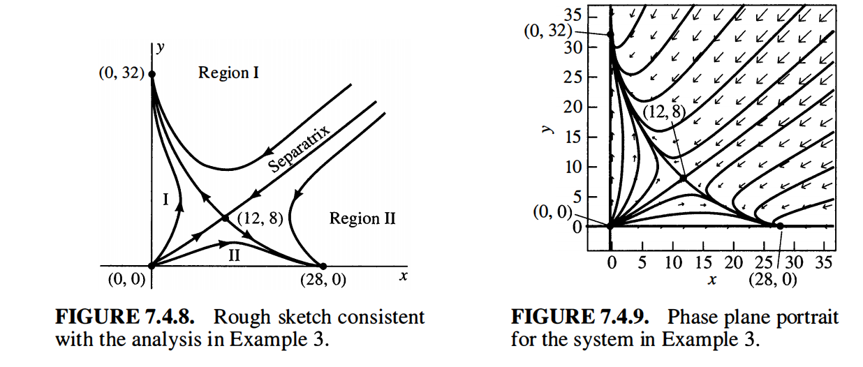
Example: coexistence impossible#

一个典型 competition system：

\begin{cases} \dot x=14x-\frac12 x^2-xy,\\ \dot y=16y-\frac12 y^2-xy. \end{cases}

它的四个 critical points 是

(0,0),\qquad (0,32),\qquad (28,0),\qquad (12,8).

线性化分析给出：

$(0,0)$ ：unstable nodal source；
$(0,32)$ ：stable nodal sink；
$(28,0)$ ：stable nodal sink；
$(12,8)$ ：unstable saddle。

于是 phase portrait 的关键结构是：

第一象限内部的 saddle $(12,8)$ ；
经过 saddle 的两条特殊轨道形成 separatrix；
separatrix 把第一象限分成两个区域。

因此：

若初值落在某一区域， $x(t)\to 0$ ， $y(t)\to 32$ ；
若初值落在另一区域， $x(t)\to 28$ ， $y(t)\to 0$ ；
精确落在 separatrix 上才会趋向 saddle $(12,8)$ ，但这在实际中几乎不可能。

所以这个系统的结论是：

和平共存不可能，最终总有一方灭绝；哪一方存活取决于初始竞争优势。

Example#

peaceful coexistence

再看另一个 competition system：

\begin{cases} \dot x=14x-2x^2-xy,\\ \dot y=16y-2y^2-xy. \end{cases}

它的四个 critical points 是

(0,0),\qquad (0,8),\qquad (7,0),\qquad (4,6).

这次局部分类为：

$(0,0)$ ：unstable nodal source；
$(0,8)$ ：unstable saddle；
$(7,0)$ ：unstable saddle；
$(4,6)$ ：stable nodal sink。

因此只要初值在第一象限内为正，轨道最终都会趋向内部的 coexistence point：

(x(t),y(t))\to (4,6).

这表示：

两种 species 可以长期稳定共存。

competition 强于 inhibition $\Rightarrow$ coexistence point 往往变成 saddle；
inhibition 强于 competition $\Rightarrow$ coexistence point 往往变成 stable sink。

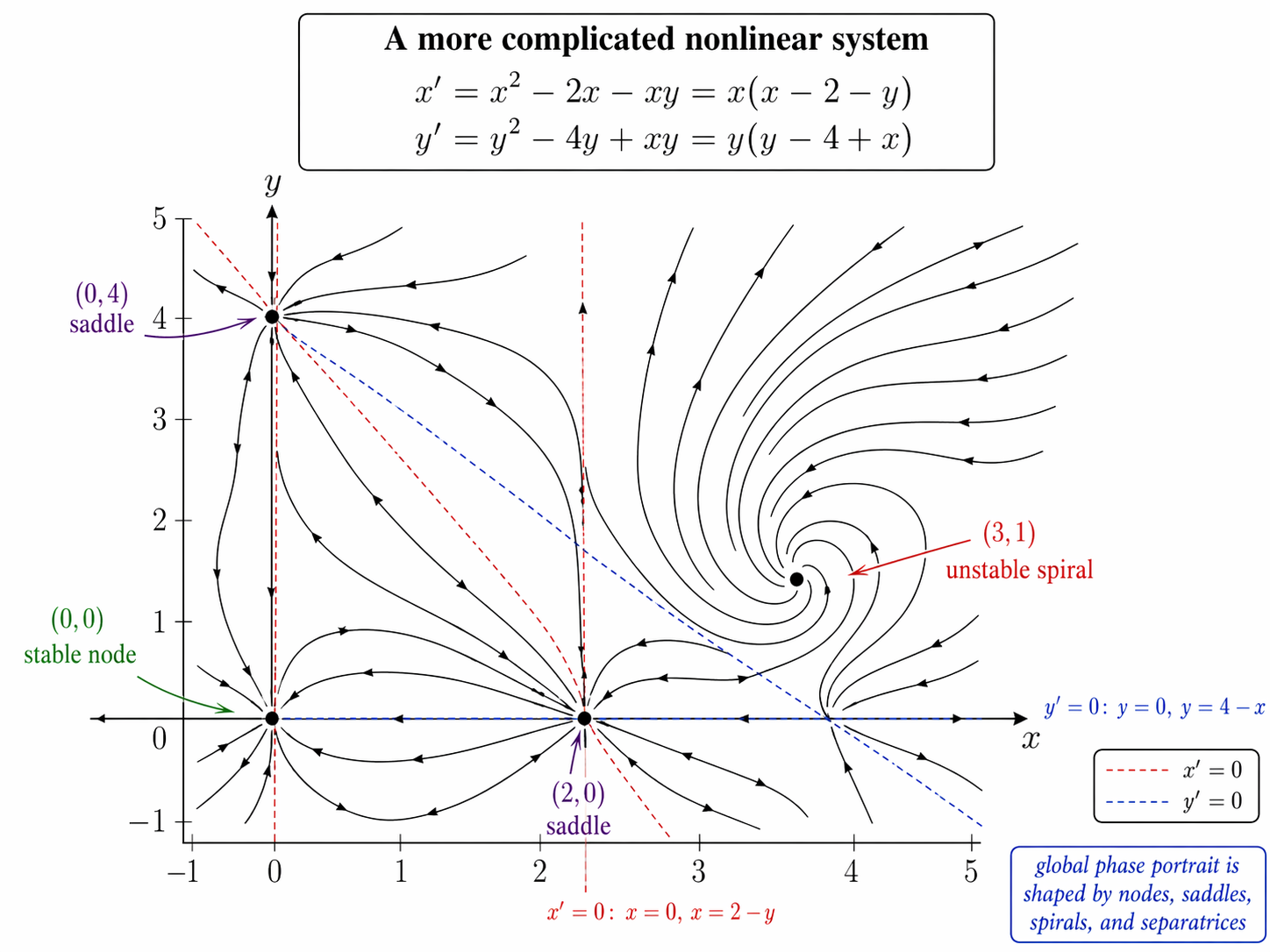
A more complicated scenario#

\begin{cases} \dot x=x^2-2x-xy,\\ \dot y=y^2-4y+xy. \end{cases}

先因式分解：

\dot x=x(x-2-y),\qquad \dot y=y(y-4+x).

Critical points#

解

x(x-2-y)=0,\qquad y(y-4+x)=0

得到四个 critical points：

(0,0),\qquad (0,4),\qquad (2,0),\qquad (3,1).

Jacobian#

Jacobian 为

J(x,y)= \begin{pmatrix} 2x-2-y & -x\\ y & 2y-4+x \end{pmatrix}.

逐点代入可得：

在 $(0,0)$

J(0,0)= \begin{pmatrix} -2&0\\ 0&-4 \end{pmatrix}

两个负特征值，所以是 stable node。

在 $(0,4)$

J(0,4)= \begin{pmatrix} -6&0\\ 4&4 \end{pmatrix}

特征值异号，所以是 saddle。

在 $(2,0)$

J(2,0)= \begin{pmatrix} 2&-2\\ 0&-2 \end{pmatrix}

特征值异号，所以也是 saddle。

在 $(3,1)$

J(3,1)= \begin{pmatrix} 3&-3\\ 1&1 \end{pmatrix}

特征方程为

\lambda^2-4\lambda+6=0,

故

\lambda=2\pm i\sqrt2.

实部为正，所以是 unstable spiral。

Qualitative picture#

因此整个系统的局部结构包含：

一个 stable node；
两个 saddles；
一个 unstable spiral。

这比前面的 textbook competition / predator-prey 图更复杂，也更能说明：

2D nonlinear system 的 global phase portrait 往往由多个 critical points 及其 separatrix 共同拼出来。